Some useful things to know about heritability (2/2)

In the previous blog post, I provided definitions of various forms of heritability. Although these definitions are pretty straightforward, there are a lot of extra things that should be kept in mind when interpreting heritability. These facts are “folk knowledge” to statistical geneticists but are often not obvious to people not working in the field. I will describe some of them below. Note that nowhere in this post will I talk about how to estimate heritability; I’m simply discussing properties of heritability, with the assumption that we have reliable ways to estimate it. I will sometimes make a distinction between different types of heritability (\(h_g^2\),\(h^2\), or \(H^2\)), otherwise the facts apply to all forms of heritability.

(1) Heritability (and also GWAS associations) come much closer to causality than you might think

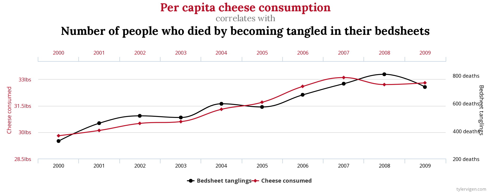
Often when we think about the proportion of variance in an arbitrary dependent variable that can be explained by arbitrary independent variables, we cannot guarantee the existence of any causal relationship between the two (even if the proportion of variance explained is high). This is the classic “correlation does not imply causation” argument. You may be familiar with plots such as the following, which show almost perfect correlations between two clearly unrelated variables:

Thus, you might reasonably think that heritability cannot be interpreted as reflecting any sort of causal effect of SNPs on a phenotype.

However, when we specifically have our independent variables represent SNP minor allele counts and our dependent variable represent a phenotype in a population of humans, then correlation DOES imply causation (with a few caveats of course; see below). This fact is quite surprising (at least it was to me when I first learned it), but it makes sense when you think about where our genetics comes from.

First, we need to understand what leads to correlation \(\neq\) causation. This phenomenon only really applies to observational (rather than experimental) data, in which we cannot control external factors from influencing our variables of interest. The main boogeymen in observational studies (which include GWAS) are confounders, which are potentially unknown factors that influence both our dependent and independent variables. Confounders can make it look as if there is a relationship between our dependent variable and independent variable even when there is none, leading us to make spurious scientific conclusions. Another problem is reverse causality, in which our dependent variable actually influences our independent variable(s) rather than the other way around.

It is serendipitous that genetic variants are basically immune to both these problems in most human populations. With regard to reverse causality, our germline genotype cannot by altered by any factors, so reverse causality is not an issue. With regard to confounders, we normally aim to address confounding via randomization, in which we delegate our independent variable to samples in a random manner that is (hopefully) independent of all possible confounders. Well, it turns out that nature has already done this randomization for us. In a population of humans, the mechanism of this randomization is meiosis followed by random mating. I won’t go into detail about how these processes work, but the consequence of these processes is that each individual basically inherits each SNP in their genome by pooling all alleles in the population together and then randomly selecting two alleles to act as their genotype - an ideal randomized experiment.

Of course, in reality you don’t inherit your SNPs from this pool of alleles independently of each other; you instead inherit a bunch of SNPs together in contiguous chunks of chromosomes, which causes SNPs physically near each other to be correlated across individuals in a population (this phenomenon is known as “linkage disequilibrium”). Moreover, in order for your genotype to truly be randomly selected from the population, individuals in the population must mate completely randomly with each other. Individuals in a homogenous population mate mostly randomly, but there are some scenarios in which they don’t. For example, people tend to mate with others in close geographic proximity (“population stratification”) or with more similar phenotypes (“assortative mating”) as themselves. This can lead to some confounding between genotype and phenotype. However, these sources of confounding are minor compared to the sort of confounders you see in other types of observational studies, and for the most part we know how control for them in human genetics studies.

Finally, let’s relate this back to heritability. The above discussion implies that we can think about the heritability of a phenotype as something akin to the total causal effect of genetic variants on a phenotype, since correlations between genotype and phenotype in a population are basically causal. This is also why in GWAS, the associations we detect are more than just associations; they are close to causal. Linkage disequilibrium often makes it difficult to pin down the exact SNP that is causal for a phenotype in a region of associated SNPs, but the fact remains that at least some SNP(s) within this region will certainly be causal for the phenotype. This is a very powerful fact.

(2) Heritability is a population-level parameter

This point is oft stated but easy to forget. Heritability is intrinsically a population-level parameter, and thus depends on the various other population-level parameters that may differ across populations. I will go into more detail about what these other parameters are in the following section.

Let’s take a moment to think about what it means to say a trait is x% heritable. This number tells us something about the average contribution of genetics to phenotypes across all individuals in the population. Perhaps we would like to know the contribution of genetics to phenotype in a given individual. However, it’s hard to say what this looks like, since everyone has a unique genotype and environment. An individual may carry a particular rare SNP with a very large contribution to their phenotype (causing their “personal heritability” to be large), but if this SNP is rare in the population, then it will not contribute much to the heritability of the phenotype in the population. In order to estimate someone’s “personal heritability”, we would have to create bunch of exact clones of the individual and raise them in a bunch of different environments, then see how much their phenotypes vary - an experiment that will obviously never happen (at least in humans). The best we can do is look for genetic effects that are consistent across individuals in a population.

(3) There is a big difference between a given SNP’s contribution to the heritability of a phenotype, and that SNP’s actual effect on the phenotype in an individual

What does it mean to talk about a given SNP’s contribution to heritability? First, some background. Recall that before defining heritability, we start out with some model for our phenotype as follows:

\[ y = f(x_1, x_2, \cdots, x_k) + \epsilon \]

where \(y\) is our phenotype, \(f\) is some function, \(x_1, x_2, \cdots, x_k\) are our minor allele counts for \(k\) SNPs, and \(\epsilon\) is whatever’s left. In practice, we almost always restrict \(f\) to be linear, in which case the model will look something like this:

\[ y = \sum_k \beta_k x_k + \epsilon \]

Here, \(\beta_k\) are coefficients for each of \(x_k\). Let’s assume that we have already centered our phenotype to mean 0, so there is no intercept term. One of the nice things about linear models is that they are easily interpretable; we can simply look at the coefficient for a given independent variable and interpret that value as its “importance” in explaining the dependent variable. Thus, we might interpret \(\beta_k\) as a given SNP \(k\)’s contribution toward explaining the phenotype. In fact, we can go beyond just saying that it “explains” the phenotype; we can let the \(\beta\)’s represent causal effect sizes of the SNPs on the phenotype.¹

Let’s walk through a concrete example. Let \(y\) represent an individual’s height in inches, centered to the population mean height. Let \(x_k\) be either 0, 1, or 2 corresponding to the number of alleles of the minor allele for SNP \(k\) (a.k.a the allele less common in the population). Thus, if \(\beta_k = 1\) for a given SNP \(k\), this means that individuals who carry one allele of SNP \(k\) will be 1 inch taller than the population average, while individuals carrying two alleles will be 2 inches taller than the population average. \(\beta_k\) can be thought of as SNP \(k\)’s actual effect on the phenotype in an individual (from the title of the section). Sometimes we call this the per-allele effect size of the SNP, or the odds ratio if our phenotype is binary.

Although the above model is very intuitive, statistical geneticists like to work with a different model when trying to estimate heritability. This model looks very similar to the above model but is in fact quite different. In particular, it is convenient to scale both \(y\) and \(x_k\) so that they have variance 1. Our new model will look like this:

\[ y’ = \sum_k \beta_k’ x_k’ + \epsilon’ \]

Although the form of the model is exactly the same as before, the variables refer to different things (since we scaled them), and thus they’re denoted with a prime symbol. In particular, \(\beta_k’\) refers to a completely different quantity compared to the intuitive \(\beta_k\) we discussed above.

Why do we scale our model in this way? It comes down to convenience. Recall that we define heritability in the following way:

\[\frac{Var(\sum_k \beta_k x_k)}{Var(y)}\]

If we scale \(y\) to have variance 1, then the denominator goes away. Meanwhile, if we scale \(x_k\) to variance 1, then the numerator just becomes \(\sum_k {\beta’}_k^2 \). Now, we have a way to interpret \(\beta_k’\) from the above model: it is the contribution of SNP \(k\) to the heritability of a phenotype.

What is the relationship between \(\beta_k’\) and \(\beta_k\)? They are in fact related by a simple formula. Assuming Hardy-Weinberg equilibrium (which is basically true for a random-mating population), \(x_k\) will follow a binomial distribution with \(n=2\) and \(p_k=\)the minor allele frequency (MAF) of the SNP (a.k.a. what proportion of total alleles in the population are the minor allele). By properties of the binomial distribution, the variance of \(x_k\) is \(2p_k(1-p_k)\). Thus, in order to scale \(x_k\) to have variance 1, we divide \(x_k\) by \(\sqrt{2p_k(1-p_k)}\) to get \(x_k’\). Because \(\beta_k x_k \propto \beta_k’ x_k’ \) (the right side should technically be divided by \(SD(y)\), but we omit this term and use the \(\propto\) symbol instead), this means that \(\beta_k’ \propto \beta_k \sqrt{p_k(1-p_k)}\), or \({\beta’}_k^2 \propto \beta_k^2 p_k(1-p_k)\).

Now we have a way to really break down what \( {\beta’}_k^2 \) (a.k.a. SNP \(k\)’s individual contribution to the heritability of the phenotype) refers to. It is proportional to the squared per-allele effect size of SNP \(k\) multiplied by \(p_k(1-p_k)\). Note that \( {\beta’}_k^2 \) depends on a population parameter \(p_k\), which is often very different in different populations. If you revisit Section (2), this is what I mean when I say that heritability depends on population-level parameters. Unfortunately, one of the confusing things that people in the field do is that they often refer to \({\beta’}_k \) as the “effect size” of SNP \(k\), even though in my opinion it’s much more natural to think of “effect sizes” in terms of \({\beta}_k \).

Why should we care about quantifying a SNP’s individual contribution to heritability in the first place? Isn’t it more direct and interpretable to just look at per-allele effect sizes \(\beta\)? Perhaps, but there are a couple reasons to care about \(\beta’ \). For one, the power to detect an association between a SNP and a phenotype in a GWAS is proportional to \(\beta’ \) rather than \(\beta\). This implies that associations involving SNPs that are common in a population (a.k.a. they have large \(p\)) are easier to detect that SNPs that are rare, even if the rare SNPs have larger per-allele effect sizes (see the following section for more discussion on this). Finally, it just comes down to convenience; it’s easier to work with \({\beta’}^2 \) instead of \(\beta^2 Var(x)\).

To summarize: when statistical geneticists talk about the “effect size” of a SNP on a phenotype in the context of heritability, they will often be referring to the effect size of the scaled SNP count on the scaled phenotype. They do this because this effect size can be conveniently interpreted as the SNP’s contribution to heritability. However, this quantity depends on population level allele frequency and is not really biologically interpretable on its own. If SNP 1 has a larger \(\beta’ \) than SNP 2, this does not imply that SNP 1 is more biologically important than SNP 2. On the other hand, the per-allele effect size or odds ratio of a SNP (a.k.a how much an individual carrying the allele will have their the phenotype change relative to population average) is biologically interpretable. If SNP 1 has a larger per-allele effect size than SNP 2, then this basically means that SNP 1 is more biologically important than SNP 2.

(4) \(h^2\) is dominated by common variants, yet rare variants have larger effects on disease than common variants.

In the last section, we established that \(h^2 = \sum_k {\beta’}_k^2 \). We also established that \({\beta’}_k^2 \propto \beta_k^2 p_k(1-p_k)\), where \(\beta_k^2\) is the squared per-allele effect size (a.k.a how much an individual carrying the allele will have their the phenotype change relative to population average) and \(p_k\) is the minor allele frequency of the SNP. Based on this formula, we can immediately see that variants with large \(p_k\) (a.k.a “common” variants) will have an outsized contribution to \(h^2\).

To give an example, suppose that we have two SNPs with allele frequencies 0.5 and 0.01 respectively. In order for SNP 2 to have the same contribution to heritability as SNP 1, it must have a per-allele effect size that is \(\sqrt{\frac{0.5(1-0.5)}{0.01(1-0.01)}} \approx 5 \) times as large as SNP 1.

Given this, it perhaps makes sense that common variants tend to explain the majority of \(h^2\), as evidenced by the fact that \(h_g^2\) estimates (which basically only include common variants) often come pretty close to \(h^2\) estimates (which include all variants) for some phenotypes. In fact, \(h_g^2\) often includes just a small subset of all common variants (for example, 500,000 out of 10,000,000 total common variants), but due to linkage disequilibrium (a.k.a correlation) between common variants, these 500,000 SNPs are able to capture most of the total effect of common variants on phenotypes.

What’s interesting is that rare variants, on average, have larger per-allele effects on disease than common variants. Long story short, this occurs due to negative selection. What is negative selection? In general, if a SNP has a large effect on any phenotype, this is bad for the individual most of the time (probably because it’s easier to break things than fix things when you randomly fiddle with the genome). It’s bad in the sense that it affects the health and most importantly the fitness of the individual. Due to decreased fitness, the individual is less likely to pass on their genetics. We call this phenomenon negative selection, and it causes the large effect SNP go down in frequency in the population and become rare.

In addition, rare variants far outnumber common variants. In part, this occurs due to random genetic drift; variants enter the gene pool via random mutations in an individual, and if the variants do not affect the fitness of the individual, they will move up and down in frequency randomly over generations, usually hanging around the rare frequency for a bit before slipping out of the gene pool unnoticed without ever reaching common frequency. Only occasionally do these variants by chance reach common frequency in the population. There is also the fact that negative selection will tend to push large-effect variants towards being rare. Depending on how large the population is, the number of rare variants can exceed common variants by 10x or more.

Despite the fact that rare variants both have larger per-allele effect sizes and far outnumber common variants, they still cannot overcome the \(p_k(1-p_k)\) term that determines their contribution to heritability, which is why common variants tend to explain most heritability.