Permutation testing is a very widely used tool to perform hypothesis testing. There already exist many resources out there that explain the procedure behind permutation testing. I’ve also performed permutation testing myself in my own research. However, for a long time I felt like I never really understood permutation tests. WHY is it valid to just permute your sample/label pairs to construct an empirical null distribution? When is this procedure not valid? How does permutation testing compare with parametric hypothesis testing, and in what scenarios would we want to use either? This blog post represents my attempt to answer these questions in a way that is both non-technical and as detailed as possible. Most of the information from this blog post was drawn from a fantastic online resource from David Howell (link here):

Overview of permutation testing

There already exist a lot of resources out there on permutation testing, so information in this section can be found basically anywhere. Permutation testing applies specifically to scenarios in which we have a predictor and label, and we would like to test the hypothesis that there is no relationship between the two things. There are scenarios in which we don’t have labels for our samples (for example, in unsupervised learning), so of course permutation testing does not apply to these settings.

The actual procedure behind permutation testing is very straightforward. In our original data, each predictor is paired with a label. We compute some test statistic from these predictor/label pairs (this test statistic should tell us something about the relationship between predictor and label). Next, we permute the predictor and label pairs. By re-computing the test statistic for each permutation, we can build a “null distribution” of test statistics. Next, we see what proportion of these null test statistics are more extreme than our observed test statistic for the original data, and this becomes our p-value. That’s it!

What should the test statistic look like? It’ll depend on what our data looks like, and what hypothesis we aim to test. For example, if our goal is to test for significant differences between two groups of samples, then a sensible test statistic is the difference in sample mean. Permutation testing can also be applied to regression setting. For example, if we want to test that the slope of a linear regression is nonzero, a sensible test statistic is the ordinary least squares estimate of the slope.

A note on hypothesis testing

Before I talk about permutation testing, I’d like to discuss some general things about hypothesis testing that help us understand why permutation testing works. In particular, what makes a hypothesis test “valid”? In frequentist hypothesis testing, all we really care about is that our hypothesis test controls type 1 error. To refresh your memory, type 1 error is false positive rate a.k.a. the fraction of truly null hypothesis that are incorrectly rejected. Why do we only care about type 1 error (rather than say type 2 error)? Well, it has to do with how we define p-values. Although p-values are very intuitive to interpret (lower p-value = more evidence against null hypothesis), the definition is somewhat technical: we say that a p-value is the proportion of test statistics more extreme than the observed test statistic UNDER THE NULL DISTRIBUTION, which equals type 1 error when rejecting hypotheses more extreme than the observed test statistic. In order to compute this p-value, we need to assume that we know what the null distribution looks like. When our estimated null distribution matches the “true” null distribution, then we say that our hypothesis test is “well-calibrated,” and we say that we have controlled type 1 error.

Wait, how do we know what the null distribution looks like? Somehow we need to estimate the null distribution from our data, even if our data is NOT actually null. This point seemed weird to me for a long time. However, this is just how frequentist hypothesis testing works. We just assume the data is coming from the null distribution even if it does not. All we care about is that IF the data actually came from the null, then our estimated null distribution would match the true null distribution. As long as this condition is satisfied, then our hypothesis test can do whatever it wants when the data comes from non-null data. In particular, any weirdness that happens when the hypothesis test is applied to non-null data will only affect power/type 2 error, which we don’t explicitly try to control (of course, it would be nice to have this quantity be as small as possible, but not a requirement). There thus exists this inherent asymmetry between type 1 error and type 2 error, which perhaps makes sense in practice: most of the time some false negatives are fine, but false positives are almost always very bad.

Permutation test vs. parametric tests

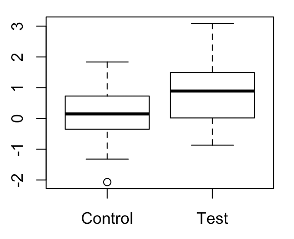
Onto permutation testing. In my opinion, the best way to understand permutation tests is to directly compare and contrast them with parametric hypothesis tests, which most of us are probably familiar with already. Let’s consider a simple example in which we have two groups of 20 values each, and we want to see whether there is a difference in means between the two groups. The values in each of these groups are drawn from a normal distribution with variance 1 and mean 0 and 1 respectively.

First, how would we perform a parametric hypothesis test between these groups? A sensible choice is the t-test. In order to perform a t-test, we need to calculate a “t-statistic.” This statistic has a numerator and denominator. The numerator is just the difference in sample means between the two groups, while the denominator is the standard error of the difference between these sample means (which we calculate by pooling the within-group sample standard deviations). We compute this statistic for our data. Assuming that the null hypothesis is true, this statistic will be distributed according to a t-distribution with n-2 degrees of freedom (where n is the total number of samples). We then look at the area under the curve for statistics more extreme than our observed test statistic, and this becomes our p-value.

Hold on, let’s think hard about exactly what our null hypothesis is here. Our null hypothesis is that our test statistic should follow a t-distribution with n-2 degrees of freedom. This requires us to make certain assumptions about our data; in this case, we assume that our data under the null are normally distributed with equal variance in both groups. Only under these assumptions will our hypothesis test be well-calibrated. There is nothing stopping us from applying a t-test to data for which these assumptions are not satisfied, but the issue becomes that our estimated null distribution will differ from the true null distribution causing our p-values to be off.

Now, let’s talk about permutation testing. Permutation testing will test a COMPLETELY DIFFERENT NULL HYPOTHESIS as our t-test. Remember that our t-test tests the null hypothesis that our test statistic follows a t-distribution with n-2 degrees of freedom. Our permutation test tests the null hypothesis that the distribution of labels is independent of group. Note that there’s no talk of a t-distribution or anything like that. Note that we don’t specify this “distribution,” we only state that it’s the same across groups. Moreover, whereas the test statistic is inseparable from the null hypothesis for the t-test, for the permutation test we don’t even specify what the test statistic looks like. The only thing we need to assume is exchangeability (a.k.a. all possible group/label combinations are equally likely under the null).

For permutation testing, the idea is that we can take basically any reasonable test statistic that can distinguish whether two distributions are different (could be difference in mean, variance, skewness, median, etc.). If two distributions are identical, then every possible statistic we could think should be identical between the two distributions. Our arbitrary choice of test statistic will thus always result in a well-calibrated test, but the power will change depending on which statistic we choose. In our case here, let’s just take the difference in means between the groups as our test statistic (seems sensible). We will permute the group/value pairs, then compute the test statistic for each permutation to construct the null distribution.

Below, I plot what the null distributions for each of these tests look like. As you can see, they are clearly different.

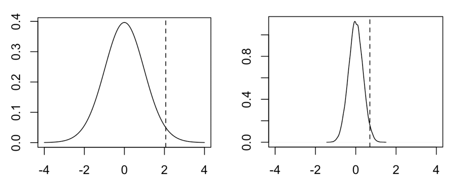
The distribution on the left is the t-distribution with 38 degrees of freedom. The distribution on the right is the empirical null distribution from permuting group/ label pairs. The test statistic for both groups is the dotted line. It turns out that in this setting, the two tests produce very similar one-sided p-values (0.023 for the t-test, 0.024 for the permutation test), though this does not need to be true in general (the two tests can differ in power as the null hypotheses they test are different). The conventional wisdom is that parametric tests are generally more powerful than nonparametric tests, though it will depend on the specific scenario. As for why parametric tests tend to be more powerful than nonparametric tests, I can only make the vague statement that we are incorporating more information into the parametric test.

In what scenarios would we prefer a permutation test? Parametric hypothesis testing requires us to make certain assumptions about our data-generating distribution that may not be satisfied in practice. For example, if we assume that our data comes from a normal distribution and it comes from a very different distribution, then we run the risk of our p-values being miscalibrated. On the other hand, for permutation testing, we only need to make the assumption that our data is exchangeable under the null (a.k.a every combination of sample/label pair is equally likely under the null). This assumption is often much easier to satisfy than the above.

Why is it valid to permute sample/label pairs to construct an empirical null distribution?

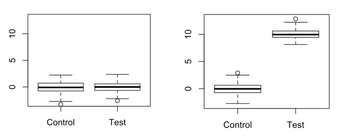
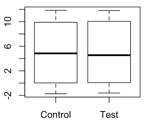
For a while, it bothered me that somehow you could construct an empirical null distribution by permuting observed labels. What if our labels are not truly generated from the null distribution? Won’t the empirical null distribution directly depend on the potentially non-null data-generating distribution? Let me give an example below. On the right, we have a scenario where there is a very large difference in mean between groups. On the left, we have a scenario that we might perceive to be the “true null” for the right scenario, where the within-group variances are the same as before but there is no difference in means between the groups.

Taking difference in sample mean as the test statistic, let’s construct empirical null distributions for each of these scenarios:

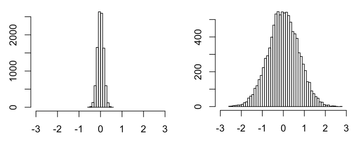
Although both distributions are centered around 0, the right distribution is clearly much more dispersed than the left distribution. How can there be such a big difference between these two null distributions? Clearly one of them is wrong. The answer is that the left scenario, though intuitive, is in fact NOT what the expected null will look like according to the permutation test; it will look something more like this:

I think this example helps illustrate the difference between parametric hypothesis testing and permutation testing. The original “null scenario” on the left represents how we would expect the data to look under the null assuming that the estimated within-group variances match the null within-group variances (which we assume to be the case if we are performing a t-test). Meanwhile, for the permutation test we make no such assumption; we assume that the pool of labels comes directly from the null distribution. This may seem weird, especially since it seems like the labels from the left scenario above better match what we assume to be the “true null.” However, this is just how permutation testing works, where we only assume exchangeability under the null. Remember that permutation testing will test a different null hypothesis as a parametric test.

Note that if we have reason to believe that estimated within-group variances match null within-group variances, then a t-test that incorporates this information will be more powerful than the permutation test (which is illustrated by the fact that the null distribution on the left is much less dispersed than the null distribution on the right).

When is it not valid to perform a permutation test?

In order for our permutation test to be well-calibrated, we must assume exchangeability of our sample/label pairs under the null. Under what conditions is this not satisfied?

A simple example in which this condition may not satisfied is in the presence of covariates. For example, suppose that we are performing a multiple regression with two independent variables:

\[y = \beta_0 + \beta_1 x_1 + \beta_2 x_2 \]

Suppose that we want to test the null hypothesis that there is no relationship between \(y\) and \(x_1\). We have to be a little careful here; note that \(y\) and \(x_1\) will not be exchangeable under the null (due to the presence of the covariate \(x_2\)). However, it will be the case that \(y | x_2 \) and \(x_1 | x_2 \) are exchangeable. How do we permute \(y | x_2 \) and \(x_1 | x_2 \)? There are actually multiple ways that we could do this. One strategy would be to just permute \(y\), but to define our test statistic to be the coefficient for \(x_1\) when regressing \(y\) on both \(x_1\) and \(x_2\). By performing a multiple regression, the coefficient for \(x_1\) is implicitly obtained from regressing \(y | x_2 \) on \(x_1 | x_2 \). Another option would be to first regress \(y\) on \(x_2\) and \(x_1\) on \(x_2\) and take the residuals directly obtain to \(y | x_2 \) and \(x_1 | x_2 \), then permute the residuals and take the test statistic to be the coefficient when regressing \(y | x_2 \) on \(x_1 | x_2 \).