This post includes some notes on frequentist vs. Bayesian inference, including discussion of both philosophical and practical differences between the two approaches to statistical inference with some concrete examples. I am still actively learning this topic so I’m sure that my understanding will progress as I revisit it in the future.
The content of this post will draw from various resources:
- Michael Jordan’s talk on Bayesian vs. Frequentist inference. https://www.youtube.com/watch?v=HUAE26lNDuE
- Andrew Gelman’s Bayesian Data Analysis textbook. http://www.stat.columbia.edu/~gelman/book/
- Notes from MIT 18.05 Probability and Statistics. http://www-math.mit.edu/~dav/05.dir/05.html
- Blog post from Jake VanderPlas on Bayesian vs. Frequentist inference. http://jakevdp.github.io/blog/2014/03/11/frequentism-and-bayesianism-a-practical-intro/
A picture to summarize everything
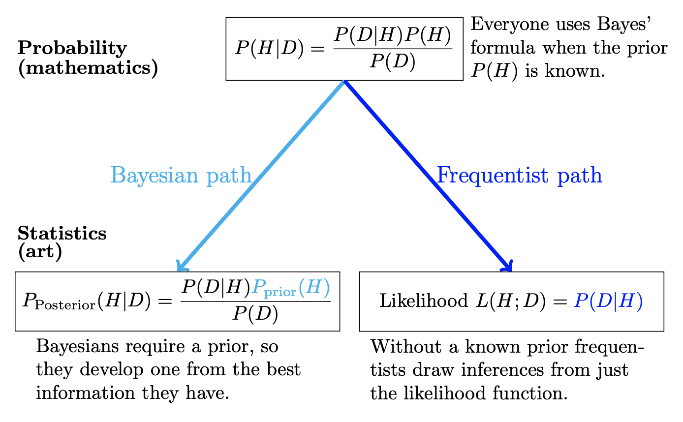
The above picture summarizes the differences between frequentist and Bayesian inference. At the top of the figure we have “probability,” which is the mathematical framework that describes how random data is generated. Meanwhile, at the bottom of the figure, we have have “statistics,” which attempts to solve the inverse problem: given observed data, it describes how to learn some feature(s) of the underlying probability model that generated the data. Whereas probability has a rigorous mathematical framework, statistics is more akin to art in the sense that there are multiple sensible solutions to the inverse probability problem, and selecting a solution is subjective.
At the top of the figure is Bayes’ rule, which is a simple mathematical fact. For example, both frequentists and Bayesians will agree that Bayes’ rule applies to settings in which a clear probability is attached to both \(H\) and \(D\), such as the following:
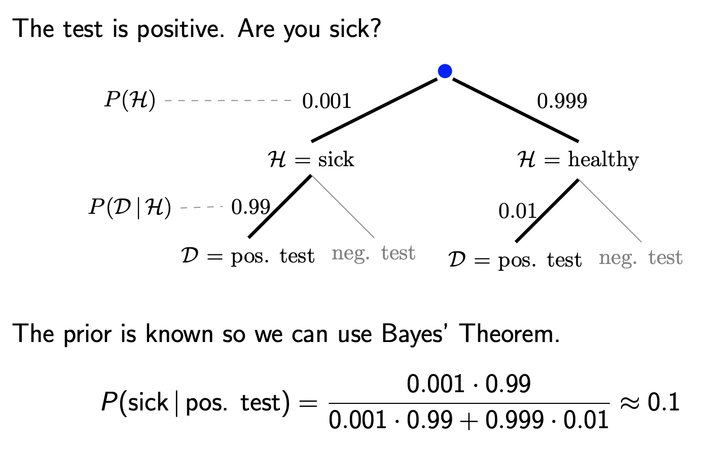
Here, \(H\) is the status of whether a person is sick or healthy, while \(D|H\) is the probability of a positive test given sick or healthy status. If we know what proportion of individuals in our populations are sick, then it makes sense to think of the quantity \(P(H)\) as this proportion, and we can compute the probability of \(H|D\) using Bayes’ rule.
However, what if \(H\) refers to a hypothesis? A hypothesis is a statement that a feature of a given probability model takes on a given value or set of values. This is where Bayesians and frequentists diverge. Both frequentists and Bayesian are perfectly happy to attach a probability to the quantity \(D|H\), which tells us how likely it is that we observe a data point given a probability model. Meanwhile, Bayesians are also happy to ascribe a probability to \(H\) itself, which reflects some subjective prior belief that the hypothesis is true. Since Bayesians think it’s valid to the think of the quantity \(P(H)\), it becomes valid to think of the quantity \(P(H|D)\) (a.k.a. the probability of the hypothesis given the data) via application of Bayes’ rule. However, to frequentists, neither the quantities \(P(H)\) nor \(P(H|D)\) make any sense, since they believe that the hypothesis is either true or false without any probability attached to it. Thus, frequentists only work with the quantity \(P(D|H)\).
Note here that probability, despite having an unambiguous mathematical foundation, is interpreted in different ways by Bayesians and frequentists. To frequentists, probability represents frequencies from repeated random experiments. This is perhaps what most people were taught probability means. For example, when frequentists say that the probability of getting heads from a coin is 0.5, this means that if we could repeatedly flip a coin an infinite number of times, the proportion of heads would be 0.5. As a result, the “likelihood” \(P(D|H)\) (a.k.a. probability of data given a hypothesis) is a sensible thing to think about, since we can repeatedly sample data from a given probability distribution. However, to frequentists, \(P(H)\) does not exist because it doesn’t make sense to repeatedly sample a given hypothesis. On the other hand, Bayesians define probability more broadly as a fundamental metric of uncertainty. For the coin example, Bayesians are fine with the frequentist view of probability. However, Bayesians also give probabilities to hypotheses, where a statement like “the probability that a parameter of a model equals x is 50%” makes sense and reflects our subjective uncertainty about the value of the parameter.
The above difference between the interpretation of probability between frequentists and Bayesians is philosophical in nature (in other words, it doesn’t have a right answer), so the comparison between frequentist and Bayesian inference should really come down to discussion of their practical differences, which I’ll go into below.
Summary of practical differences
So, what are the practical differences? Because Bayesians attach probabilities to hypotheses whereas frequentists do not, this seems like it should certainly affect inference. In frequentist statistics we can’t make statements like “this hypothesis is probably true”; we can
The first thing I should mention is that frequentist and Bayesian inference often lead to very similar conclusions for simple problems.
Walking through an example
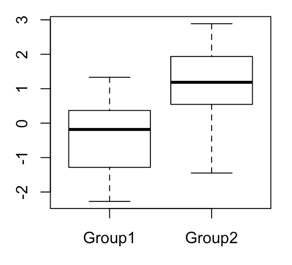
To illustrate the differences between frequentist and Bayesian inference, I’ll describe a specific example in which we have two groups and would like to learn something about the difference in means between the groups. Let’s say that both groups have values drawn from a normal distribution with \(\sigma^2 = 1\), while group 1 has \(\mu_1 = 0\) and group 2 has \(\mu_2 = 1\). Each group has 20 values total.
For simplicity, let’s assume that we known \(\sigma^2\) a priori. There are several things we might want to do with the quantity \(\mu_2 - \mu_1\). One thing would be to estimate \(\mu_2 - \mu_1\) as best as possible, and give some uncertainty about our estimate of \(\mu_2 - \mu_1\) in the form of a confidence interval. Another different thing would be to perform hypothesis testing, in which we see whether our data is more consistent with a given null model (for example, that \(\mu_2 - \mu_1 = 0\)) or an alternative model. I will talk about both these things in both the frequentist and Bayesian frameworks.
Both frequentist and Bayesian methods start out with a likelihood \(P(D | H)\), which describes the probability that we observe a data point given a probability model. In this case, the likelihood is given by the PDF of the normal distribution:
\[ p(x | \mu, \sigma) = \frac{1}{\sigma \sqrt{2\pi}} e^{-\frac{1}{2}(\frac{x - \mu}{\sigma})^2}\]
As you can see, the PDF for the normal distribution depends on two parameters: \(\mu\) and \(\sigma\). In our case, we are dealing with two normal distributions (one for each group), so our likelihood function will consist of the PDFs of two normal distributions multiplied together.
Estimation
First, let’s suppose that we would like perform estimation of the parameter \( \mu_2 - \mu_1 \).
Frequentist approach. In the frequentist approach, we only work with the likelihood. A standard way to estimate a parameter in frequentist world is via maximum likelihood estimation (MLE), which selects a value of a parameter that maximizes the likelihood function. Maximum likelihood estimation has nice properties, which is why people like to use it a lot. For example, it is consistent (which means that as the number of samples increases, the MLE will converge to the true value of the parameter), efficient (since it achieves the lowest mean squared error of all consistent estimators of a parameter), and asymptotically normal (meaning that the distribution of the MLE will converge to a normal distribution as the number of samples increases). Note that these properties are all frequentist in nature, as they describe the behavior of our estimator when repeatedly collecting data. Without going through the derivation, the maximum likelihood estimate of \( \mu_2 - \mu_1 \) in our case will simply be \( \hat \mu_2 - \hat \mu_1 \), where \( \hat \mu_1 = \frac{\sum_n x_n}{n} \) represents the sample mean of samples in group 1 and likewise for \(\hat \mu_2\).
We would also like to attach some uncertainty to our MLE estimate. Because our MLE estimate is a function of random data, it will also be random itself and have a distribution. In our case, because our data is normally distributed, \( \hat \mu_2 - \hat \mu_1 \) will also be normally distributed with mean \( \mu_2 - \mu_1 \) and variance \(\frac{2 \sigma^2}{n} \), where \(n\) is the number of samples in a given group (this can be readily computed by using properties of the normal distribution). In general, with more complicated likelihood functions, it’s usually not that simple to compute the exact distribution of a maximum likelihood estimator. In these scenarios, people often rely on the asymptotic normality of the MLE. It can be shown that with increasing samples, the distribution of the MLE of some parameter \(\theta\) converges to a normal distribution with mean \(\theta\) and variance \(\frac{1}{nI(\theta)}\), where \(I(\theta)\) is the Fisher information of \(\theta\) and \(n\) is the number of samples. For even more complicated scenarios, we can approximate the sampling distribution of the MLE using non-parametric resampling approaches such as the bootstrap or jackknife (I’ll get to these methods in a few sections).
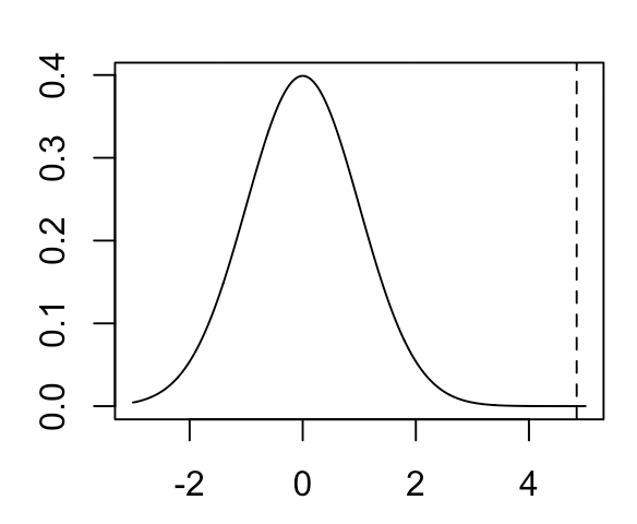
In our case, the true distribution of our MLE estimate of \( \mu_2 - \mu_1 \) (which we cannot observe) will look like the following:
\( \hat \mu_2 - \hat \mu_1 \) for our particular example is indicated by the vertical line. Recall that the only thing that we know is \( \hat \mu_2 - \hat \mu_1 \) and \(Var (\hat \mu_2 - \hat \mu_1) \) (assumed to be known a priori). We don’t actually know the true mean of the distribution. How do we turn these things into some metric of uncertainty on our estimate of \( \mu_2 - \mu_1 \)? We do this by constructing a confidence interval. Suppose we want to construct a 95% confidence interval. We do this by taking the region \(\pm 1.96 * SD( \hat \mu_2 - \hat \mu_1 )\) around \( \hat \mu_2 - \hat \mu_1 \), which will look like the following:
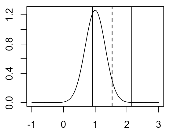
It seems perfectly natural and intuitive to report our point estimate of \( \mu_2 - \mu_1 \) along with an estimate of the variance of this point estimate in the above fashion. However, if we would like to define exactly what our confidence interval represents, we need to be a bit careful. The definition is as follows: if we were to repeatedly sample our data and construct a confidence interval in this manner each time, then 95% of the time our confidence interval would include the true value of \( \mu_2 - \mu_1 \). This definition may seem convoluted, but it’s simply what comes out when we report the MLE and variance of sampling distribution of the MLE together in this fashion.
There are some additional important things to note here. When thinking about confidence intervals, we are implicitly considering many data sets that we have not actually seen. In other words, when stating that the confidence interval we constructed will include the true value of \( \mu_2 - \mu_1 \) 95% of the time, we are saying that among all possible data sets of sample size 40 with group 1 drawn from a normal distribution with mean \( \mu_1 \) and variance 1, and group 2 drawn from a normal distribution with mean \( \mu_2 \) and variance 1, then 95% of confidence intervals we construct from each of these data sets will cover the true value of \( \mu_2 - \mu_1 \) (which happens to be 1 in our case, though we don’t know this from just our data). The notion of averaging over unobserved potential datasets is ubiquitous in frequentist inference and absent from Bayesian inference, so this is one of the key aspects in which the two fields differ. I’ll revisit this point in a bit.
Bayesian approach. In the Bayesian approach, we work with both the likelihood and the prior, which is a distribution over potential values of our parameter that quantifies our degree of belief in each of the potential values. Although we can let our prior distribution take any form, it is typical to select a prior that is a conjugate prior of our likelihood (which means that it “pairs well” with the likelihood in some way, see below).
In Bayesian inference, we estimate a parameter by constructing a posterior distribution for the parameter, which is the likelihood multiplied by the prior divided by the marginal likelihood (a.k.a. \(P(D)\)). Note that we obtain the marginal likelihood by integrating over \(H\) as follows: \(P(D) = \int_H P(D | H) P(H)\). What should our prior distribution look like? It turns out that when the likelihood follows a normal distribution, selecting a prior that follows a normal distribution will result in a posterior that is also normally distributed. For this reason, it’s convenient for us to select a prior that follows a normal distribution. In general, with more complicated likelihood functions, it’s often not possible to select a prior that will result in a posterior distribution with a simple form. In these scenarios, we can use Markov Chain Monte Carlo (MCMC) methods to efficiently sample from the posterior distribution, though I won’t go into how these methods work.
Let’s say that we have very little prior knowledge of what \( \mu_2 - \mu_1 \) should look like. In this situation, it would be reasonable to choose a prior that is evenly spread out over many values, such as a normal distribution with mean 0 and variance 100. Skipping over the derivation, our posterior will look like a normal distribution with mean \(\frac{1}{\frac{1}{\sigma_0^2} + \frac{n}{\sigma^2}} ( \frac{\mu_0}{\sigma_0^2} + \frac{\sum_n x_n}{\sigma^2} ) \) and variance \( ( \frac{1}{\sigma_0^2} + \frac{n}{\sigma^2} )^{-1} \), where \(\mu_0\) and \(\sigma_0^2\) are the mean and variance of our prior and \(\sigma^2\) is the (assumed to be known) variance of the likelihood. Just to provide some intuition on what these quantities represent, the posterior mean is essentially a weighted average of the prior mean and the sample mean, where the weights are determined by the reciprocal of the prior variance and sample variance respectively. Meanwhile, the posterior variance is essentially a weighted average of the sample variance and prior variance. If the prior variance is very large (indicating little prior knowledge), then our posterior mean and variance will be determined mostly be the sample mean and variance.
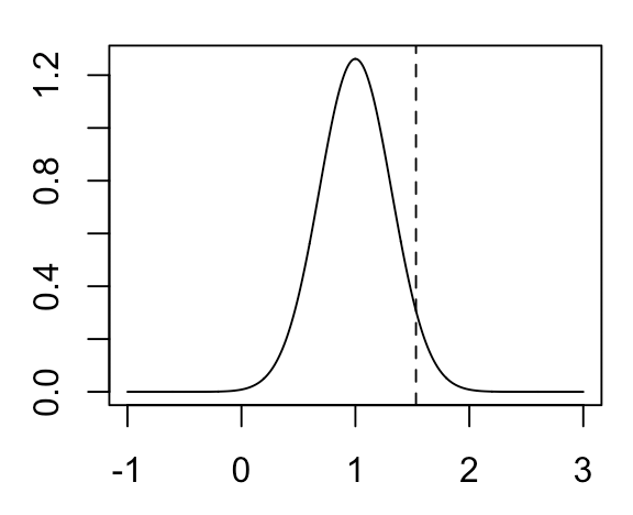
For the scenario in which our prior has mean 0 and variance 100, our posterior distribution for \( \mu_2 - \mu_1 \) will look like the following:
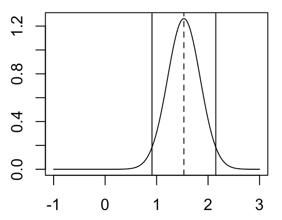
If we want to produce a single point estimate of our parameter from this posterior distribution, the typical thing to do is the take the maximum a posteriori (MAP) estimate, which is the mode of the posterior distribution (indicated by the dotted line). Meanwhile, to provide some information on the uncertainty of this point estimate, often we will specify an x% credible interval around that point estimate (95% credible interval indicated by the solid lines), which is an interval within which the parameter has an x% chance of falling. Note that the MAP estimate and 95% credible interval shown here are nearly identical to the MLE estimate and 95% confidence interval shown above. This occurs because we selected an uninformative prior, so our posterior is dominated by the likelihood. The credible interval is perhaps more intuitive than the confidence interval, and in fact it’s a common mistake to assume that an x% confidence interval is the interval within which the parameter has an x% chance of falling (which is actually the definition of the credible interval). However, the similarity here between the confidence interval and credible interval under an uninformative prior demonstrate that perhaps it is valid to think of a confidence interval as something like the above definition.
What if we have strong prior knowledge about the value of \( \mu_2 - \mu_1 \)? Suppose that for whatever reason, we have a strong reason to believe that \( \mu_2 - \mu_1 \) is close to 0, in which case we specify a prior distribution for \( \mu_2 - \mu_1 \) that has mean 0 and variance 0.01. In this case, the posterior will look like the following:
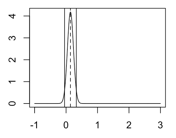
As you can see, due to our high amount of prior certainty about the value of \( \mu_2 - \mu_1 \), the posterior is much closer to 0 (though our observed data has shifted this distribution slightly away from 0).
Given that we can select our prior in any way we want (resulting in any sort of posterior), there is a certain amount of trust going into the scientist to select a prior that actually reflects their true uncertainty about the parameter of interest. In the above example, we would need to provide strong justification for why we expect \( \mu_2 - \mu_1 \) to be so close to 0. It is also probably reasonable to try multiple different priors and see if the posterior changes greatly. One perhaps nice thing is that as we gather more samples, the posterior will be dominated by the likelihood rather than the prior, in which case our choice of prior will not really affect the posterior.
Note that in contrast to frequentist inference, at no point during Bayesian inference do we think about data sets that we haven’t observed. In Bayesian inference, our posterior is conditioned on the observed data set, and all conclusions we draw about our parameter apply specifically to the data set at hand. On the other hand, recall that an x% confidence interval is all about data sets that we haven’t observed: it states that x% of confidence intervals constructed from all possible datasets from our model will include the true value of the parameter. Although this particular distinction between Bayesian vs. frequentist inference (a.k.a. frequentist considers unobserved data sets; Bayesian considers only the data set at hand) is philosophically interesting, it’s unclear to me whether there’s any practical utility to thinking about them in this manner (especially since Bayesian and frequentist approaches give very similar results with an uninformative prior as shown above).
Non-parametric frequentist approach. Both previous approaches have required that we specify the likelihood \(P(D | H)\). What if we don’t actually know this likelihood? This scenario comes up frequently in genomics, in which our observed quantity of interest (such as the expression levels of a gene) can have a complicated distribution affected by many technical and biological factors that are challenging to model. In this scenario, we turn to non-parametric approaches that enable us to estimate the sampling distribution of our estimator without actually specifying the likelihood. The typical way we would do this is via bootstrapping, which involves resampling from our observed data (with replacement), computing our estimator from the simulated data, and looking at the distribution of the estimator across these simulated datasets. The bootstrapped distribution of \( \hat \mu_2 - \hat \mu_1 \) looks like the following:
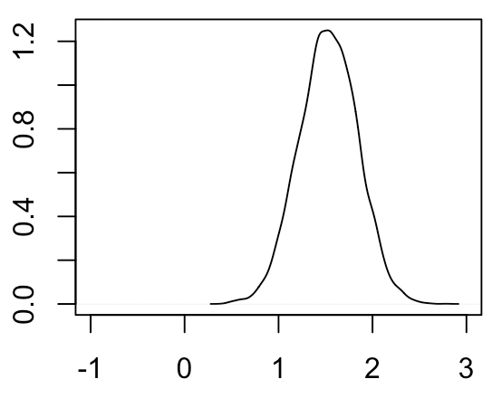
As you can see, this distribution looks very similar to both the sampling distribution of the MLE and the posterior with an uninformative prior. In our case, because we know the likelihood function for our data and can easily compute the sampling distribution of the MLE, it doesn’t really make sense to bootstrap. However, if for example our data was drawn from an unknown distribution that deviates substantially from a normal distribution, then the bootstrapped distribution of \( \hat \mu_2 - \hat \mu_1 \) would still be valid whereas the sampling distribution of the MLE and posterior assuming a normal likelihood would not be valid.
Bootstrapping is frequentist in the sense that no prior is placed on the parameter of interest, and the goal is to estimate the sampling distribution rather than the posterior of the parameter. As far as I know, there isn’t really a widely used Bayesian counterpart to bootstrapping (there indeed exists something called the Bayesian bootstrap, but I’ve never seen it used in practice before).
One final point: bootstrapping is perhaps more straightforward than parametric estimation because it enables us to easily estimate the sampling distribution of any arbitrary statistic that is a function of our data. For example, instead of taking the difference of sample means as our statistic, we could take the difference in sample medians, or difference in range, etc. Without a model, we aren’t really concerned about the bias or consistency of our estimator; we simply use our best judgement to pick a statistic that seems reasonable for our problem at hand. Some people might argue that we need to specify a model in order for our problem to be well-formulated, but the truth is that often in genomics we can easily define a reasonable statistic for our biological question at hand without specifying a model for our data. Bootstrapping is used due to its simplicity.
Hypothesis testing
I have previously described the frequentist (both parametric and non-parametric) and Bayesian approaches to estimation of the quantity \( \mu_2 - \mu_1 \). A different form of information comes from hypothesis testing, in which we typically try to quantify evidence for a null hypothesis (in our case, that \( \mu_2 - \mu_1 = 0 \)), then decide whether we want to reject this null hypothesis or not.
Frequentist approach. In the frequentist approach to hypothesis testing, we again work with only the likelihood. Again, our statistic of interest will typically be the maximum likelihood estimate of our parameter. The idea behind frequentist hypothesis testing is to basically just treat the data as if it was generated under the null hypothesis, then see how “unexpected” our MLE is. We quantify this level of unexpectedness using the p-value, which tells us what proportion of data sets drawn from our null distribution result in estimates of our parameter that are more “extreme” than our observed estimate.
There are several different ways we can compute p-values. One common way is the Wald test, which simply takes the MLE and the standard error of the MLE (either computed analytically or using the asymptotic properties of the MLE), then computes a statistic \( \frac{\hat \theta - \theta_0}{SE(\hat \theta)} \) (where \(\hat \theta)\) is the MLE of our parameter and \(\theta_0\) is the value of our parameter under the null hypothesis). This statistic will be asymptotically distributed according to a standard normal distribution. In our case, the null distribution of the Wald test statistic will look like the following:
where the vertical line is our observed test statistic. As you can see, this value is quite extreme relative to the null distribution and results in a one-sided p-value of 1.07e-5.
Another common test is the likelihood ratio test, for which the test statistic is written like \( -2 \ln ( \frac{\sup_{\theta \in \Theta_0} \mathcal{L}(\theta)}{\sup_{\theta \in \Theta} \mathcal{L}(\theta)} ) \). \(\Theta\) represents the full set of possible values that the parameter \(\theta\) can take, while \(\Theta_0\) represents a subset of \(\Theta\) that represents our null hypothesis (often this will be just a single value of \(\theta \), such as \(\theta = 0\)). \(\sup_{\theta \in \Theta_0} \mathcal{L}(\theta)\) represents the likelihood of our data when selecting a value of \(\theta\) from \(\Theta_0\) that maximizes this likelihood, while \(\sup_{\theta \in \Theta} \mathcal{L}(\theta)\) represents the likelihood when selecting a value of \(\theta\) from \(\Theta\) (a.k.a. the entire parameter space) that maximizes the likelihood. Under the null, the likelihood ratio test statistic will be distributed according to a \(\chi^2\) distribution with degrees of freedom equal to the difference in degrees of freedom between \(\Theta_0\) and \(\Theta\). For example, if our null hypothesis is \(\theta = 0\) and the alternative hypothesis is \(\theta \neq 0 \), the difference in degrees of freedom will be 1. Although the likelihood ratio test and Wald test are asymptotically equivalent, for finite samples the likelihood ratio test will tend to be more powerful. In particular, for simple hypotheses (in which both the null and alternative hypothesis involve the parameter taking on a single value), the likelihood ratio test is the most powerful test according to the Neyman-Pearson lemma, which is often used to justify the use of the likelihood ratio test.
To complete the trio of classical approaches to hypothesis testing, the score test (or Lagrange multiplier test) is another alternative to likelihood ratio/Wald testing, but from my experience seems to be less commonly used in practice so I won’t talk about it.
Note that all frequentist hypothesis tests operate by assuming that our data is generated from the null hypothesis even if it is not. This assumption is built into our definition of the p-value, which refers to the proportion of test statistics generated from the null that are more extreme than our observed test statistic. There is thus this asymmetry between the null distribution and the alternate distribution in frequentist hypothesis testing, where we really only care about controlling type 1 error (false positive rate) rather than type 2 error (false negative rate). In other words, as long as our hypothesis test produces “well-calibrated” p-values (a.k.a. our model for the null matches the true null) IF the data was generated from the null, it can do whatever it wants if the data is not generated from the null.
Also note that frequentist hypothesis testing is consistent with frequentist notion of averaging over unobserved data sets, as I discussed above. The p-value refers to
Bayesian approach.
In the Bayesian approach to hypothesis testing, the pivotal quantity to estimate is the Bayes factor rather than the p-value.
Non-parametric frequentist approach.
When should we use each method?
Given that frequentist approaches are generally more prevalent in science than Bayesian approaches, I think that for tradition’s sake one should prefer taking a frequentist approach when there is no clear advantage to taking a Bayesian approach (though it will depend on the field). For example, most biologists (including myself) are only taught frequentist methods, and I think that there is a significant barrier to entry to learn Bayesian methods from scratch. Below, I’ll describe some scenarios in which we might prefer one approach over the other.
Good prior information
In the scenario where we have good prior information about our parameter, it seems like a no-brainer to take a Bayesian approach. However, one thing to keep in mind is that at the limit of infinite sample size, the posterior will be completely dominated by the likelihood, in which case it will converge to the same distribution as the sampling distribution of the MLE (see the Bernstein-von Mises theorem). Thus, when we have data sets with a very large amount of samples, unless we have very strong prior information about our parameter of interest, the output of Bayesian and frequentist methods will likely be similar.
No good prior information
Without informative prior information, Bayesian and frequentist methods will produce basically the same results for simple problems (as illustrated above). However, note that sometimes simply specifying a prior (which can be uninformative a.k.a. it might be flat across many possible values of our parameter) will change the way we approach a particular problem.
One example is in the handling of nuisance parameters. Normally
Another important example in which an “uninformative” prior actually modeling complicated hierarchical problems. Hierarchical problems arise when we have many parameters in a model that are related to each other in some way. For example, we might be performing a regression with a large amount of predictors in which can think of the coefficients as drawn from some common distribution. By modeling the coefficients as coming from the same distribution, we implicitly apply a form of “shrinkage” of the individual parameters toward the global mean of the distribution, which can be advantageous in many ways (for example, if the individual parameters estimates are very noisy on their own). Whereas it is often natural to think of hierarchical models in Bayesian inference, in frequentist inference it is typically much less straightforward to do so.
For a concrete example, consider the scenario of differential expression analysis between two conditions across many genes (say 100).
There is additionally an approach known as empirical Bayes which aims to learn
Unknown likelihood function
In the scenario that it is challenging to define the likelihood for our data (or if it’s complicated to analytically compute the standard error of the MLE), it is natural to pursue non-parametric resampling approaches such as the bootstrap or jackknife. This scenario is actually quite common in genomics, so it should be viewed as meaningful benefit of frequentist inference over Bayesian inference (which requires at a minimum the specification of a likelihood).