Synopsis

The main result from our recent paper is that we’ve managed to make Perturb-seq much cheaper to run (around an order of magnitude over existing strategies), using a combination of new experimental and computational strategies. The experimental strategies involve only minimum changes to the standard Perturb-seq protocol that do not add additional labor or equipment requirements. Our new way of running Perturb-seq also increases power to learn genetic interaction effects, which you can essentially learn “for free” from the same data.

   

Detailed summary

What is Perturb-seq?

Perturb-seq (aka CROP-seq, CRISP-seq) is a type of ‘genetic screen’ that was developed around 2016. Genetic screens are experiments in which you modify the genetics of some model system (e.g. human cells in a dish, a fly, a mouse, or something else), then see how the model system changes to learn something about how genetics affects biology.

Perturb-seq uses a molecular tool called CRISPR to modify the genetics of cells in a dish in a precise manner. Then, it uses a technique called “single-cell RNA-sequencing” to read out the expression levels of all ~20,000 genes in each individual cell. Based on how gene expression levels change across the entire genome in response to specific genetic perturbation(s) in each cell, we can learn about the relationship between specific genes and complicated gene expression networks that underlie many cellular processes.

History and context of Perturb-seq

To make genetic modifications to model systems, people originally used X-rays or various chemicals to randomly induce genetic mutations. Subsequently, various molecular tools like RNA interference made it possible silence specific genes’ expression. Most recently, CRISPR has become the tool of choice to make precise edits wherever you want in the genome.

After making genetic perturbations in your model system of choice, the next step is to measure some phenotype in the model system. There are lots of possible phenotypes to measure, which depend on the model system. The model system in which Perturb-seq is typically applied is a ‘cell line,’ which comprises cells (usually human or mouse) with some modifications so the cells can survive in a dish. Cell lines have been used for many years in all sorts of research and drug development settings. For cell lines, the possible phenotypes to measure include cell growth/survival, morphology, expression of certain genes, and many others.

Historically, there has been a trade-off between the complexity of the phenotype being measured, and the throughput of the genetic screen for the phenotype. For simple (a.k.a one-dimensional) phenotypes like cellular fitness, it has long been possible to test and learn the effects of many hundreds or thousands of genetic perturbations in a single pool of cells. The way this works is through a ‘pooled screen,’ where you put all your perturbations (when using CRISPR, these are viruses that each carry a single instruction or ‘sgRNA’ to target a specific genetic region) on the cells all together. Then, you put the cells through some ‘selection procedure’ that is related to the phenotype you’re measuring - for example, if you want to test the effects of genetic perturbations on growth/fitness, you can just let the cells grow; if you want to test the effects on the expression of some marker gene, you can sort the cells based on the expression of the gene; etc. Finally, you can measure the relative change in the proportion of each perturbation before vs. after applying the selection procedure. If you see, for example, that the relative proportion of perturbations targeting gene A has gone up after the cells are allowed to grow for a while, then you can conclude that gene A is a ‘negative regulator’ of cellular fitness/growth (because knock-out of gene A results in increased growth). 

Although it’s relatively easy to learn the effects of many genetic perturbations on simple one-dimensional phenotypes like fitness, these simple effects unfortunately don’t tell you anything about the complicated molecular processes that underlie all human disease. What if we instead want to measure perturbation effects on a complex, high-dimensional phenotype? One commonly-studied example of this is a ‘gene expression profile’ (a.k.a. the expression levels of all ~20,000 genes in the genome), which is measured through RNA-sequencing and gives you a lot of information about transcriptional networks in the model system. Unfortunately, it’s not possible to measure high-dimensional phenotypes using the pooled strategy described above because we cannot select for values of a high-dimensional phenotype in our cell population. Instead, the perturbations have to be applied one-at-a-time to pools of cells that are physically separated from each other (in different wells of a plate, or separate plates), then separately measuring the high-dimensional phenotype in each pool of cells. This greatly limited the throughput of this type of genetic screen.

In 2016, Perturb-seq was introduced. It was one of the first types of genetic screens that managed to combine pooled screening with a high-dimensional phenotype (specifically, gene expression profiles). It accomplished this by introducing clever barcoding strategies that enable you to measure gene expression profiles for individual cells using single-cell RNA-sequencing, while also detecting which genetic perturbations (from CRISPR) are present in each individual cell from the barcodes. This obviated the need to apply any sort of selection filter to the cells. In a Perturb-seq experiment with a single pool of cells, you can learn the effects of many hundreds or thousands or genetic perturbations (from CRISPR) on the expression levels of all ~20,000 genes. This is a lot of data and has enabled some interesting biological discoveries that were not found in simpler screens. One cool example is from this paper from 2022, which conducted a massive genome-wide Perturb-seq screen (targeting ~10,000 genes) and discovered (among many other things) a new subunit of the Integrator complex, which is a highly-conserved gene complex involved in RNA processing in all animals. There is still a lot of biology to be learned out there, even in systems that we think we understand well.

Main drawback of Perturb-seq (and ways to fix it)

Unfortunately, even though Perturb-seq enables you to run a pooled genetic screen in a single pool of cells (thus greatly reducing cost and labor requirements compared to the one-at-a-time approach), it is still constrained by cost. Roughly speaking, around 100 cells need to be sequenced to learn the effects of one genetic perturbation, which costs around $100 in total. Thus, it would cost on the order of $1,000,000 to conduct a Perturb-seq screen at the same scale as the one in Replogle et al. 2022 (mentioned above). This cost is way too high for almost all academic labs, which prevents Perturb-seq from being applied more widely.

The high cost of Perturb-seq primarily stems from the large amount of sequencing that needs to be done for many 100,000s or millions of cells. There are several ways to reduce this cost. One approach is to reduce the cost of the sequencing using new fancy technologies. Another approach is to reduce the number of cells that need to be sequenced. The latter approach is the one that we opted to focus on in our work. The nice thing about these two approaches is that they are fully independent, and thus can be paired with each other to obtain multiplicative cost decreases. However, we did not use any new sequencing technologies in our study.

How Perturb-seq works currently

In order to describe how we decreased the cost of Perturb-seq, we need to first go through the current experimental protocol of Perturb-seq. A diagram is shown below.

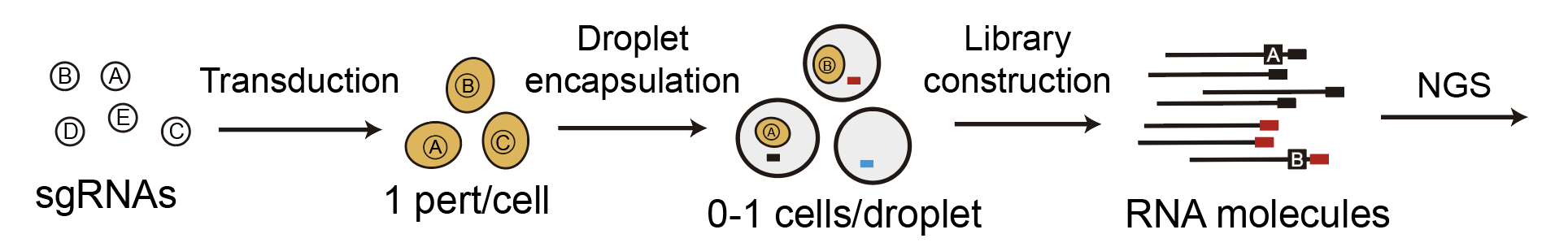
We start out with a pool of viruses that each contain an sgRNA, which is basically an instruction that tells a protein called Cas9 where to cut the genome. Next, we ‘transduce’ a pool of cells with the virus. In other words, we put the viruses on the cells all together, then the viruses will randomly infect the cells and integrate their genomes with the cells’ genomes. The concentration of virus (also ‘multiplicity of infection’ or MOI) is calibrated so that most of the cells will either not be infected at all, or are infected by exactly one virus. Following transduction, we can get rid of all the cells that were not infected, since we include a fluorescent marker or antibiotic resistance gene in the virus that enables us to select for only infected cells.

Next, we encapsulate the infected cells in special tiny water-in-oil ‘droplets’ by putting the cells in a microfluidic device (this is a standard step in droplet-based single-cell RNA-sequencing). The cells are loaded into the device at a low concentration so that only one cell at a time enters each droplet. In practice, this results in most droplets being empty. Each droplet contains a bead covered with barcodes that labels every RNA molecule in the droplet with the barcode. Previously, we also designed the virus in a way so that the sgRNA actually gets transcribed, which enables us to read out which sgRNAs are present in a given cell. Finally, the barcoded RNA molecules across all droplets get combined together and sequenced using next-generation sequencing technologies.

What we changed

From the ‘standard’ Perturb-seq protocol described above, each set of reads we sequence from a given droplet captures the RNA expression levels of one cell containing one perturbation. What if we could simultaneously measure the effects of multiple perturbations in multiple cells? 

This is the underlying idea behind our approach (which we call ‘compressed Perturb-seq’). It turns out that with very small modifications to the standard Perturb-seq protocol, you can generate droplets that capture either individual cells containing multiple perturbations, or multiple cells containing one perturbation. This is illustrated below.

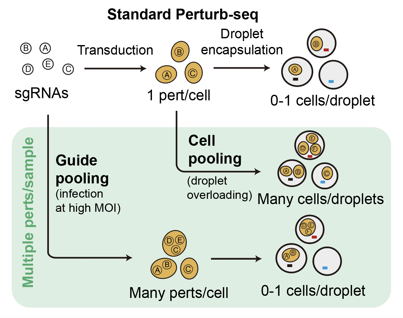
At the top is the standard Perturb-seq protocol. By simply increasing the concentration of virus when transducing cells (a.k.a. infecting the cells at ‘high MOI’), you end up with multiple random viruses that infect each cells, and thus multiple random genetic perturbations per cell. We call this approach ‘guide-pooling.’ Meanwhile, by simply increasing the number of cells when loading the microfluidics device, you end up with multiple cells that enter each droplet, as well as many fewer empty droplets. We call this approach ‘cell-pooling.’

After doing cell-pooling or guide-pooling, each droplet will capture multiple perturbations rather than one. However, the effects of the perturbations are mixed together in a sort of confusing way. If we were to directly sequence the droplets generated from cell-pooling, we would end up measuring something like the average expression of all genes across the multiple cells present in the droplet. Meanwhile, if we were to directly sequence the droplets generated from guide-pooling, we would end up measuring the expression of a cell containing multiple perturbations.

Though not immediately obvious, it turns out that we can directly learn the effects of individual perturbations from these measurements without any additional work. Moreover, we can actually learn these effects with far fewer of these special measurements than the standard approach. There is a rich theory from a field called compressed sensing that exactly describes the conditions under which we can learn individual perturbation effects from measurements of multiple perturbations. Omitting all the technical details, compressed sensing theory suggests that we can greatly reduce the number of measurements needed to perform Perturb-seq given the following three things:

1. Measurements represent random sums of perturbation effect sizes

For cell-pooling, we can show (relatively straightforwardly) that measurements corresponding to the average expression levels of cells containing one perturbation each are equivalent (after a simple transformation) to the average of effects of each of the perturbations, which is effectively the same as a sum.

For guide-pooling, it’s somewhat less straightforward to show that measurements corresponding to expression levels of one cell with multiple perturbations is equivalent (after a simple transformation) to the sum of effects of each of the perturbations. This requires the non-trivial assumption that the effects of individual perturbations will tend to combine additively when multiple perturbations are in the cell. However, we observed empirically in our data that this assumption holds.

I should note that the presence of genetic interaction effects may appear to violate this assumption, but it doesn’t necessarily. Due to the fact that each cell contains an essentially unique combination of perturbations, then genetic interaction effects will “average out” when looking across all cells (and thus not violate this assumption), so long as the interaction effects are equally positive and negative in number/magnitude.

2. Perturbation effect sizes exhibit certain ‘structure,’ in the sense that they can be fully represented with a small number of latent parameters

Compressed sensing theory tells us that our perturbation effect sizes need to have particular latent structure for us to accurately learn them from a small number of sums of effects. We can pretty confidently say that this structure is present in all Perturb-seq datasets. This structure is illustrated below: 

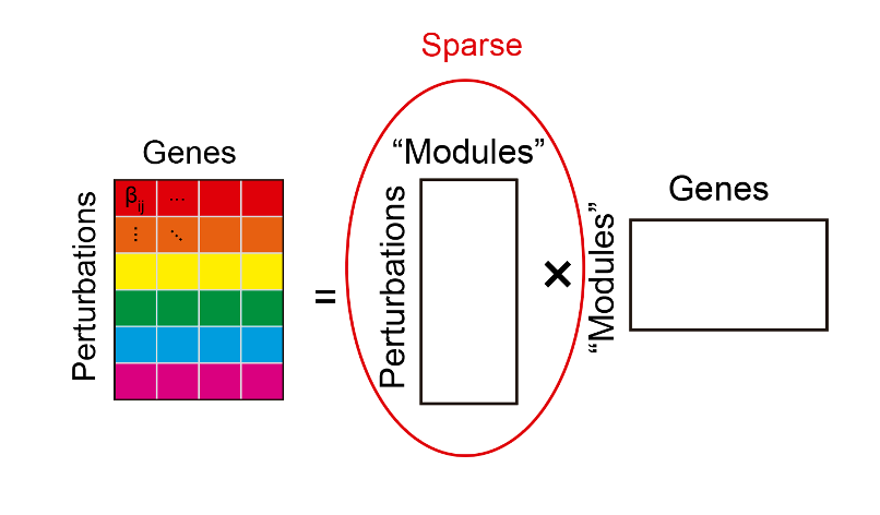
On the left, we have a matrix corresponding to the perturbation effect sizes we aim to learn. Each row corresponds to the effects of a single perturbation on the expression levels of all genes. The structure that needs to be present in this matrix is shown on the right.

For one, it needs to be possible to decompose the matrix into two ‘factor matrices’, where the number of columns of the left matrix (rows of the right matrix) is small. If we think about what this means biologically, it’s that genes’ expression tends to be organized into a small number of ‘modules,’ and perturbations act on modules as a whole rather than on individual genes. Do we expect this structure to be present in our data? Yes; everything we know about the behavior of gene expression suggests that it should be the case. Gene expression is tightly co-regulated, and it’s been observed in virtually every gene expression dataset that a small number of latent modules can describe the behavior of all genes’ expression.

The second and last condition is that the left factor matrix needs be ‘sparse’ (a.k.a most entries are zero). This means that most perturbations do not affect most modules. It’s been observed in many previous CRISPR screens that most genetic perturbations don’t affect the phenotype of interest, so we can fairly confidently predict that this condition will be true for Perturb-seq data as well.

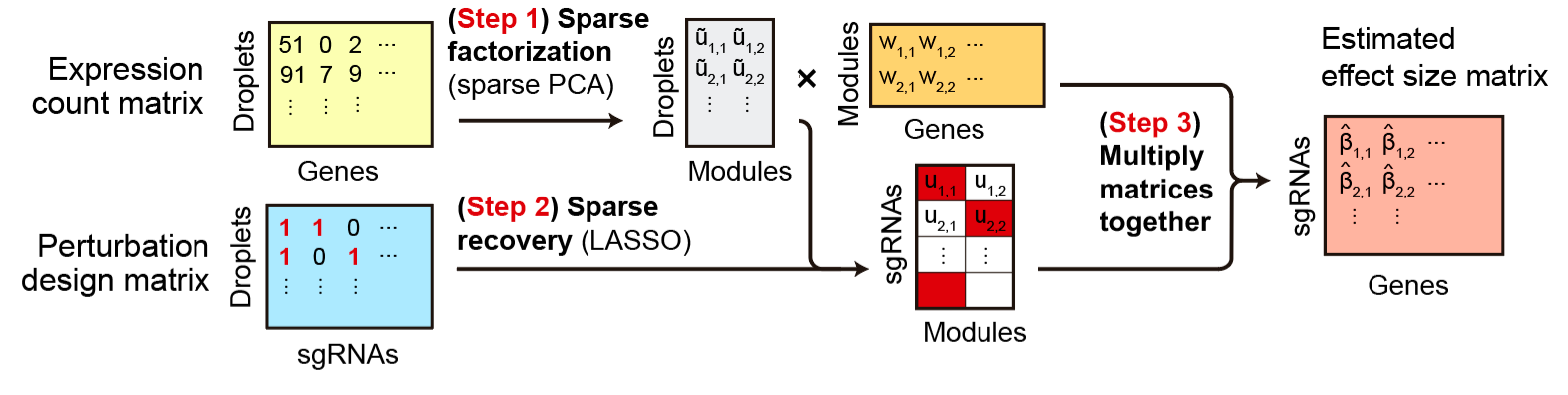
3. Specific algorithms (such as the factorize-recover algorithm) are used to infer perturbation effects from the special measurements

Motivated by this requirement, we adapted the factorize-recover algorithm to work with Perturb-seq data (see below). We called our method ‘FR-Perturb’ (factorize-recover for Perturb-seq). I won’t go into detail about what the algorithm does, but just know that theory says that we can get good performance (in terms of accurately inferring effect sizes from a small number of special measurements) when we use this algorithm.

Compressed Perturb-seq works

We tested cell-pooling and guide-pooling, together with inference using FR-Perturb, in a series of Perturb-seq screens in THP-1 cells (a human macrophage cell line) treated with bacterial lipopolysaccharide (LPS), which induces the ‘innate immune response’ in these cells. We selected this model system primarily out of convenience, since this project was started by Brian Cleary in the Regev lab which has previously worked with this model system or closely related ones (Parnas et al. 2015, Dixit et al. 2016). Also, the innate immune response (in particular the TLR4 pathway) is one of the most well-characterized pathways out there, with decades of research dedicated to studying it, so we could check if the system responded in ways that were expected based on previous knowledge.

We selected 598 immune-related genes from various sources to perturb. Then, we implemented both cell-pooling and guide-pooling in two separate screens targeting these 598 genes. For each of these screens, we also ran a standard Perturb-seq screen (targeting the same genes) to act as validation. An outline of the experimental design of our study is shown below:

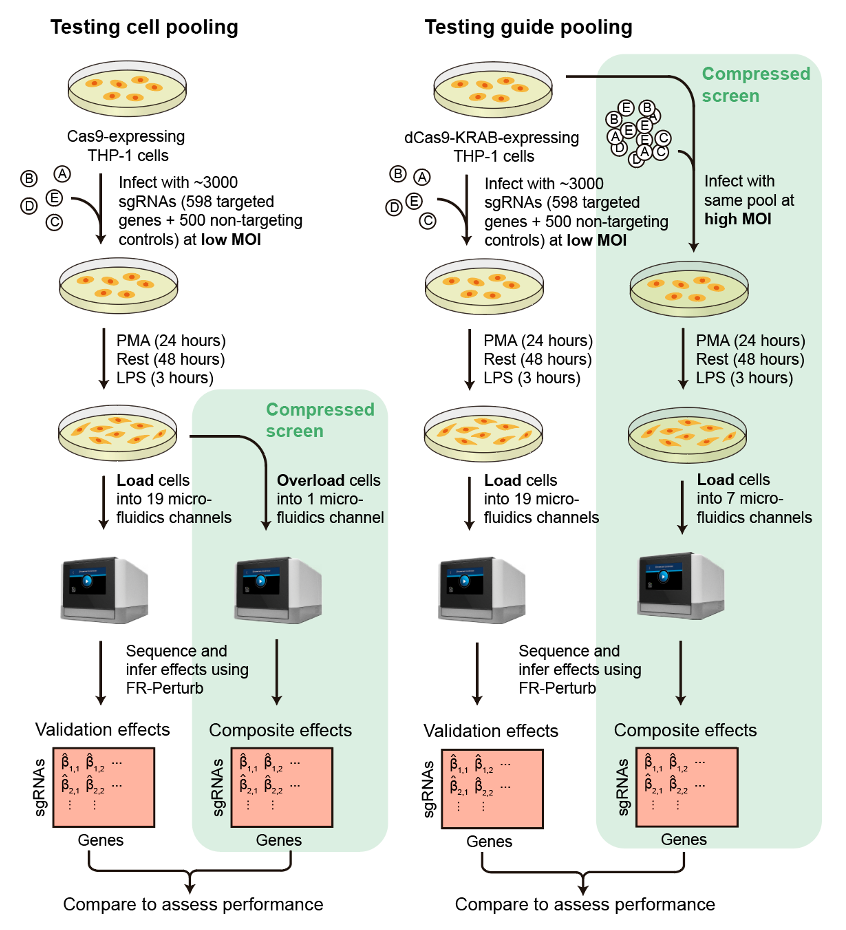
We found that cell-pooling works great. This is shown qualitatively by the heatmaps representing perturbation effect sizes below.

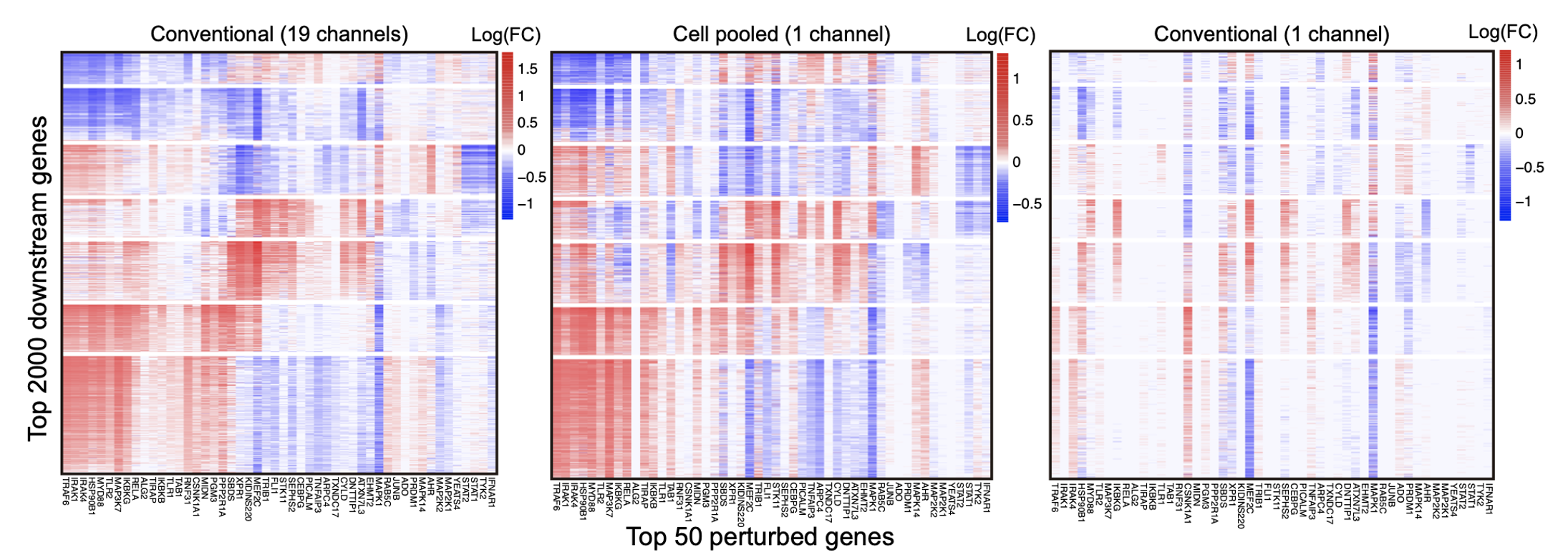
The leftmost plot represents the perturbation effect sizes (log-fold changes of expression levels) learned using FR-Perturb from the full standard Perturb-seq screen (columns = top 50 perturbations with the strongest overall effects on all genes, rows = top 2,000 genes whose expression changes the most across all perturbations). This screen used a total of 19 microfluidics ‘channels’ (which you can think of as a physical unit of a microfluidics device). The middle plot represents the same perturbation effect sizes learned from only 1 microfluidics channel using cell pooling. For comparison, the effect sizes learned from 1 microfluidics channel following the standard protocol is shown in the rightmost plot.  As you can see, we can recapitulate the effect size patterns from the full 19 channel standard screen with only 1 cell-pooled channel.

We also found that guide-pooling works quite well. This is shown qualitatively by the heatmaps below.

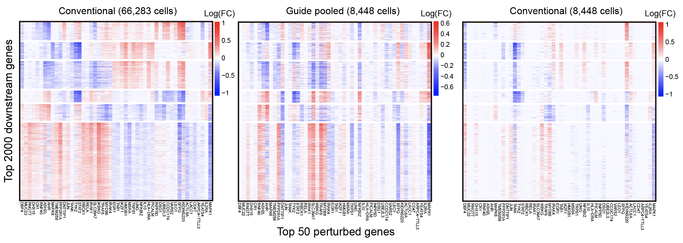
The leftmost plot represents the perturbation effects learned using FR-Perturb from a full standard screen with 66,283 cells, while the middle plot represents the same perturbation effects from only 8,448 cells generated from guide-pooling.

Quantifying efficiency gains of compressed Perturb-seq

To give a more quantitative answer to how much better compressed Perturb-seq does than standard Perturb-seq, we held out half of our standard Perturb-seq data, then looked at the correlation between effects learned from the compressed Perturb-seq screens with the held-out data (aka computed its out-of-sample validation accuracy). We compared this with the out-of-sample validation accuracy of the remaining standard Perturb-seq data. The results are shown below (left: cell-pooling, right: guide-pooling).

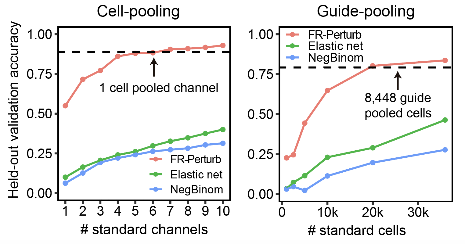
There are quite a bit of details that need to be clarified with these plots. We randomly downsampled the remaining standard Perturb-seq screen to learn the relationship between sample size (x-axis) and out-of-sample accuracy (y-axis) of the standard screen, and to see where it intersects with the out-of-sample accuracy of the cell-pooled or guide-pooled screen (dotted line). Out-of-sample accuracy represents the correlation of the top \(n\) effects (where \(n\) = the total number of significant effects in either the cell-pooled screen for the left plot or the guide-pooled screen for the right plot when performing inference with FR-Perturb) with the same effects in the held-out data. \(n\) was on the order of 10,000 effects in both screens (or around 0.1% of 598 * 20,000 = ~10,000,000 total effects). Significance was defined as FDR q-value < 0.05 computed from p-values computed from permutation testing.

There are also three lines per plot, corresponding to the out-of-sample validation accuracy when inferring effects using FR-Perturb and two other previously-used inference methods for Perturb-seq data (elastic net regression (Dixit et al. 2016) and negative binomial regression (Gasperini et al. 2019)). For each line, the same method was used to perform inference in both the out-of-sample validation screen and the in-sample comparison screen, to ensure a fair comparison. It’s actually also possible to infer effects from the cell-pooled/guide-pooled screen using these two other methods, but these results are not shown here (the dotted line is from inference with only FR-Perturb).

What do we conclude from these plots? From here, you can see that cell-pooling performs equivalently to 4-6x as many channels of standard Perturb-seq when performing inference with FR-Perturb in both the out-of-sample validation and in-sample data (red line in left plot), while guide-pooling performs equivalently to ~2.5x as many cells from standard Perturb-seq (red line in right plot). These numbers actually undersell the performance of compressed Perturb-seq, because part of our new approach is the use of our new computational method FR-Perturb to infer effects. Thus, when reporting the “cost reduction” of compressed Perturb-seq, we compare the dotted line to the higher of the green and blue lines (in this case the green line, which represents the out-of-sample validation accuracy of the standard Perturb-seq data when performing inference with elastic net regression, matching what Dixit et al. 2016 did). Because the dotted line (aka the full cell-pooled/guide-pooled screens) far exceeds the highest point in the green line (at x = 10 channels in the left plot or ~33k cells in the right plot), we downsampled the cell-pooled/guide-pooled screens until we found the point in which their out-of-sample accuracy intersected with the highest point in the green line. This point ended up being ~1/5 of a channel from the cell-pooled screen and ~3,000 cells from the guide-pooled screen. From these numbers, we computed the accuracy-matched cost reduction of compressed Perturb-seq. This ends up being a 20x reduction for cell-pooling (we give a lower bound of 4x when taking the whole cell-pooled channel instead of 1/5 because it’s technically not possible to subdivide a channel in practice), and a 10x reduction for guide-pooling.

An important non-obvious conclusion regarding FR-Perturb

There’s a hidden conclusion here, which I think can be easily overlooked when reading the paper (unfortunately). It’s that previous inference approaches for Perturb-seq, which learn perturbation effects on each gene’s expression one gene at a time, seem to be pretty bad. As shown in the above plot, if you take a standard Perturb-seq dataset, randomly split the samples in half, then compare the correlation of the top 0.1% of effects between the two halves inferred with previous methods, the correlation of the effects is under 0.5. On the other hand, if you do this and infer effects with FR-Perturb, you get a correlation of ~0.9. In fact, the observed performance gains of compressed Perturb-seq over previous approaches is primarily just driven by inference with FR-Perturb, rather than the experimental changes (though the experimental changes still help).

Why does FR-Perturb perform so much better than other approaches? The main difference between FR-Perturb and things like elastic net regression or negative binomial regression is that FR-Perturb first learns a small number of gene “modules” capturing co-regulated groups of genes, then infers perturbation effects directly on the modules, rather than on individual genes as the other methods do. This has a strong de-noising effect (individual genes’ expression is very noisy especially at the single-cell level), which results in much better consistency of effects across independent subsets of Perturb-seq data. It’s still true that cell-pooling/guide-pooling lead to better performance than the standard experimental protocol when inferring all effects with FR-Perturb, just not “order-of-magnitude” good (at least in our current study; it may be possible in future studies with a greater number of perturbations/cell than we attained).

It’s interesting that the factorize-recover algorithm, which on paper is needed to most efficiently learn effects from compressively-sensed data, ends up far out-performing existing methods even when applied to non-compressively-sensed data due to its hidden de-noising properties. This isn’t something that we foresaw before running these experiments, but serendipitous findings are common in science I guess.

Of course, there are several important caveats to be made with the analysis in the above plots. The biggest one is that consistency of effects between subsets of data does not guarantee that the effects are “real”; they could just be consistently wrong across the subsets. We ran many analyses that tried to independently show that effects learned with FR-Perturb are “better” than the effects learned with other methods (such as looking for known effects of certain perturbations), finding the FR-Perturb does seem to be better than these other methods in these analysis. However, to be honest we don’t know the exact ground truth Perturb-seq effects, and all these analyses are a noisy approximation to the truth. We also tried hard to repeat all these analyses while varying various ‘arbitrary’ parameters, like the number of effects being compared when computing out-of-sample validation accuracy, how we compute out-of-sample validation accuracy (Pearson vs. Spearman correlation, sign concordance, etc.), and other things. None of these changes resulted in substantially different results, which is a good sign.

Guide-pooling enables you to learn genetic interaction effects

One added bonus of guide-pooled data is that because cells have multiple guides, you can learn genetic interaction effects for free. A “genetic interaction effect” can be defined as the effect of a combination of perturbations in a sample that is “not explained” by the individual effects of “lower-order” combinations of perturbations. This definition is left purposely vague because basically every paper has a different definition for what it means for an effect to be “explained” by lower-order combinations of perturbations (it’s a bit of a mess, but that’s for another discussion). 

We focused on second-order interaction effects in our paper, which have a somewhat more consistent definition. A second-order interaction effect between a pair of perturbations is the phenotypic effect of the two perturbations in a sample that differs from the sum of the effects of the individual perturbations. Unfortunately, when we tried to infer individual second-order effects from our guide-pooled screen, we did not find any significant effects (due to the small size of the guide-pooled screen, which was really only designed to learn first-order effects).

However, we were still able to detect something like interaction effects using a different strategy, as illustrated in the plot below.

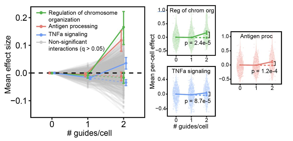
We grouped together perturbations based on their known function. The x-axis represents cells that contain 0, 1, or 2 of any perturbations in a given group (each group is connected by a line in the plot). The y-axis represents the mean change in gene expression in each cell group for genes in one of several “gene programs” (groups of genes with similar function). Interaction effects were defined as a deviation of the mean effect in the 2 perturbation/cell group from 2*mean effect in 1 perturbation/cell group. Significance of interaction effects was assessed by permutation testing. This is all a little convoluted but we only had adequate power after making these groupings.

Rest of paper

There are number of other results in the paper that focus on the biology we learned from our Perturb-seq screens. These results are less generally applicable so I won’t go into them.

Some non-obvious conclusions

Here are some other important conclusions from the paper that may not be obvious from a cursory read.

1. The cost reductions reported in our study are far from optimized and are specific to our model system

In our study, we only really tried one specific level of “pooling” (a.k.a. number of perturbations per measurement) for both cell-pooling and guide-pooling. For cell-pooling, we ended up measuring around 1.9 cells per droplet on average (compared to 1.1 from the standard approach), though with many more non-empty droplets per channel (33,000 vs. 4,000). For guide-pooling, each cell ended up with an average of 2.5 perturbations (compared to 1.1 perturbations from the standard approach). The degree of pooling was somewhat random; we simply tried to get as high a number as possible. Despite our efforts, these numbers were still somewhat low.

How can we improve on these numbers? We learned that getting more cells into each droplet for cell-pooling will (surprisingly) not necessarily lead to better performance (see below for more discussion), so it’s not exactly clear how to improve our implementation of cell-pooling. However, in the case of guide-pooling, we observed that performance reliably scaled with the number of perturbations per cell; we saw the best performance with cells containing 4 or more perturbations (the highest number for which we had enough cells to still infer effects). Thus, getting more perturbations into each cell will likely lead to higher cost reductions than observed in our study. Unfortunately, this leads to some other technical issues, as cells start to die when they get separately infected by too many viruses. This can likely be mitigated by the use of Cas12 arrays (which enables multiple genes to be knocked out with a single virus), but we did not do anything like that in our study.

Also, there is the obvious idea: why not combine cell-pooling and guide-pooling together? This is certainly feasible because they modify completely independent steps in the experimental protocol. However, in theory, it’s hard to infer effects from the resulting combined cell/guide-pooled measurements (droplets containing multiple cells each with multiple perturbations) because perturbation effects combine differently for measurements generated from cell-pooling vs. guide-pooling. Nonetheless, in practice, it may very well be possible to combine cell-pooling and guide-pooling together and still accurately learn the effects somehow. The only way to be sure is to try.

To summarize, the cost reductions reported in the study should be seen as a starting point rather than an optimized number. Our study should be viewed as a proof-of-concept that cell-pooling and guide-pooling, even in their un-optimized state, can lead to large cost reductions. By further optimizing guide-pooling and/or combining guide-pooling with cell-pooling, it may very well be possible to attain an additional order of magnitude (or even larger) decrease in cost.

2. Cell-pooling actually does worse than the standard approach on a per-droplet basis, but this is offset by obtaining many more non-empty droplets per channel

When cell-pooling, we obtained ~33,000 non-empty droplets from a single channel, compared to ~4,000 non-empty droplets per channel from the standard protocol. Droplet-for-droplet, cell-pooling actually does worse than the standard 1 cell/droplet approach (surprisingly), but you get so many more non-empty droplets per channel that it ends up being overall a net efficiency gain. Because there are so many more non-empty droplets per channel, you need to sequence them more deeply (we did 4x higher sequencing coverage for the cell-pooled channel than a corresponding standard channel). This makes it a little more complicated to compute the cost reduction of cell-pooling, but we included the extra cost of sequencing when doing so.

The performance of cell-pooling is hard to predict for the above reasons. Simply loading more cells into the microfluidics device is not guaranteed to further reduce your costs. You will get more non-empty droplets (good), but each droplet will also contain more cells (bad). It might be surprising that more cells per droplet is bad thing - isn’t that what the compressed sensing stuff is all about? However, it makes sense when you realize that each additional cell present in a droplet increases the noise of the expression measurement relative to the effect size of the perturbation (this is kind of a confusing point that is discussed in the supplement of the paper). This increased noise offsets the gains from observing multiple effects per droplet. Thus, cell-pooling only outperforms the standard approach by exploiting a quirk of how cells are encapsulated in droplets, rather than by measuring multiple perturbations at a time per se. 

On the other hand, guide-pooling is simpler. We observed that the performance of guide-pooling scaled proportionally with the number of perturbations/cell. This makes sense in light of the fact that noise in expression does not increase with more perturbations/cell (whereas noise does increase with more cells/droplet in the case of cell-pooling). Moreover, the per-channel sequencing costs are the same for guide-pooling as they are for the standard approach. Figuring out how to introduce more perturbations per cell will likely reduce costs even more than attained in our study. Plus, you get to learn genetic interaction effects for free. For all these reasons, we are more optimistic about the use of guide-pooling than cell-pooling in future studies.

3. Even if you want to just run Perturb-seq the normal way (aka without the experimental changes we propose), our results suggest that you can benefit from (1) not discarding droplets with multiple cells and/or cells with multiple perturbations, and (2) inferring effects using FR-Perturb rather than other methods.

Our results have several important implications for existing screens, or for future screens that are conducted according to the standard protocol.

For (1), the standard protocol will, by chance, already generate a number of droplets containing multiple cells or cells containing multiple perturbations. These droplets are usually discarded from analysis, but our results suggest that you should not do so. You can keep these droplets to increase the effective sample size of your experiment.

For (2), we showed that FR-Perturb far outperforms (based on out-of-sample validation accuracy) other methods (elastic net regression, negative binomial regression) even when applied to standard Perturb-seq data. As mentioned above, this performance gain stems from the FR-Perturb inferring perturbation effects on de-noised gene modules rather than on very noisy individual genes.