Authors: Julia Domingo, Guillaume Diss & Ben Lehner
Synopsis
In this paper, the authors constructed \(5184\) distinct genotypes for the arginine-CCU tRNA in yeast, corresponding to all possible combinations of alleles in 7 different extant yeast species. They measured epistatic effects on fitness across all orders. They found that epistatic effects across all orders are prevalent, as well as some interesting relationships between epistatic effects and the structure of the tRNA (e.g. 2nd and 3rd order effects were more likely to be negative if all mutants were on the same strand; 2nd order effects were more likely to be positive if they restored Watson-Crick base pairing, etc.).
Summary
Figure 1a-c
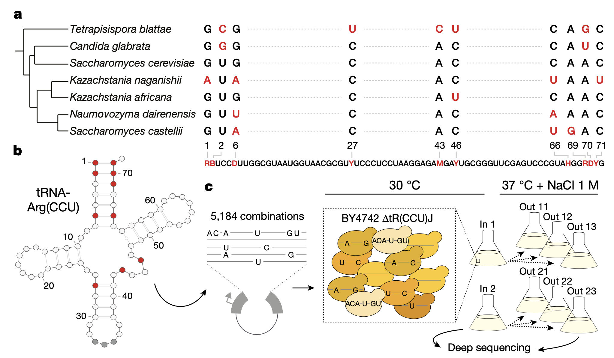
1a: Shown are the different variants of the arginine-CCU tRNA (tRNA-Arg(CCU)) in 7 different yeast species. In total, there are 10 base pairs within this gene that differ across species. 6 of those base pairs have 2 different alleles and 4 of them have 3 different alleles.
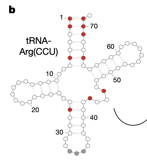
1b: Structure of the tRNA-Arg(CCU). Variable positions across species are indicated in red.
1c: In total, there are \(2^6 \times 3^4 = 5184\) possible genotypes that can be constructed from all alleles across these 7 species. Each genotype is separated from one another by at most 10 base pairs. The authors synthesized all genotypes and transformed them into S. cerevisiae (strain BY4742). The authors conducted 6 replicate selection experiments to quantify the fitness of all genotypes under restrictive conditions (high temperature and salt). After filtering, 4176 genotypes remained.
Figure 1d-e
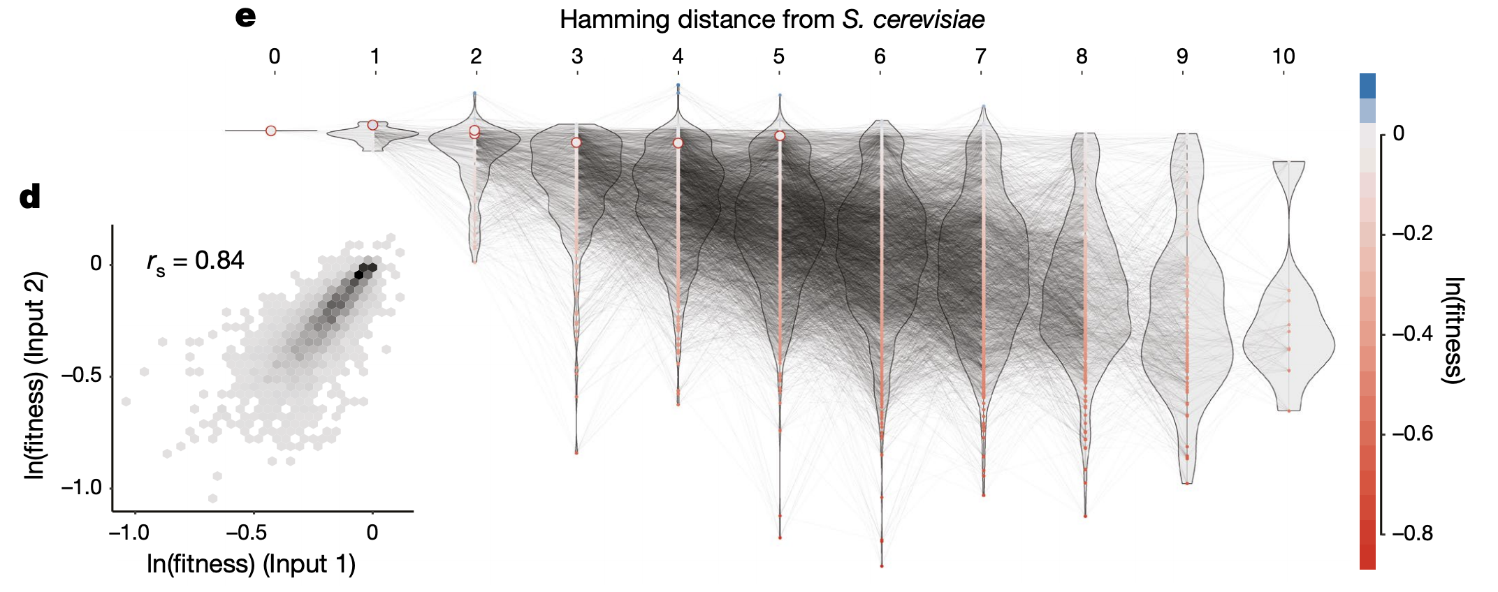
1d: Correlation in log(fitness) values for filtered genotypes across 2 replicate transformation experiments. Fitness for each genotype was computed by taking the log ratio of read proportion before vs. after selection.
1e: log(fitness) of all genotypes stratified by number of differing base pairs vs. S. cerevisiae. The red circles are the fitness values for the 7 yeast species.
Figure 2
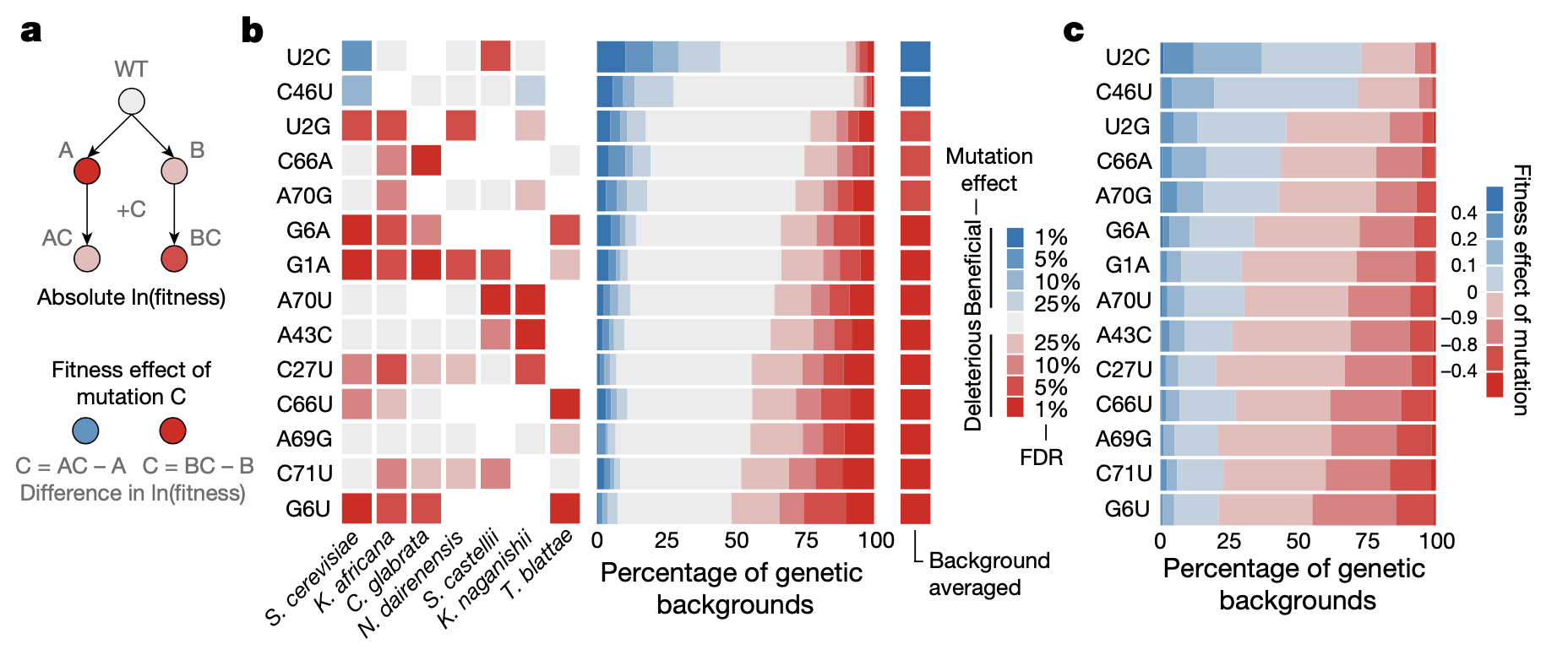
2a: The effect of mutation C on fitness can change depending on whether the sample already contains mutation A or B. This would be evidence of epistasis between A and C, B and C, or both.
2b: Left: Significance (in FDR) of effect of 14 possible single-nucleotide substitutions (y-axis) in 7 different yeast species (x-axis). Color indicates the direction of the effect. Note that all mutations can be either detrimental or beneficial depending on the genetic background. Right: Significance of effects of the 14 single-nucleotide substitutions (y-axis) across all genetic backgrounds.
2c: Same plot as 2b Right, but showing effect size rather than significance.
Figure 3a
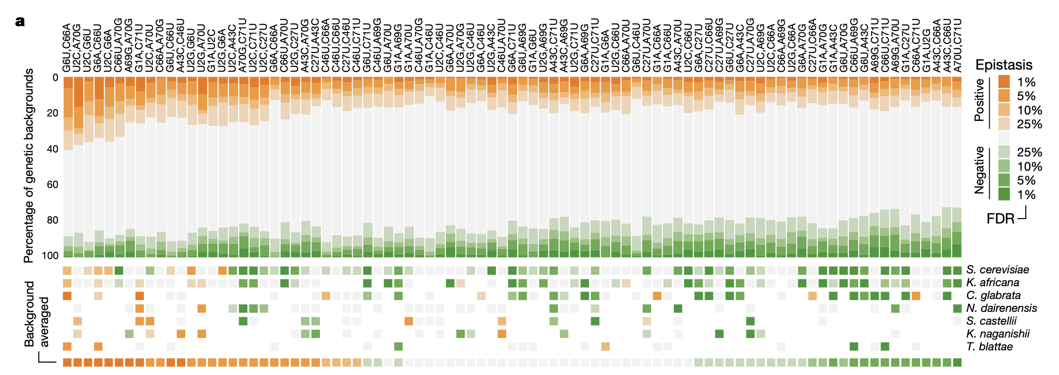
3a: Significance of epistatic effects of 87 possible pairs of mutations across all genetic backgrounds (top) and 7 different yeast species (bottom). Pairwise epistatic effects were computed by taking the difference in the log(fitness) between the pairwise mutant vs. expected phenotype (sum of 1st order effects on log(fitness)).
What’s interesting is that most pairwise epistatic effects are negative in the yeast species, but across all genetic backgrounds they are basically equally negative and positive. This might have something to do with the fact that most of the yeast species have high fitness relative to the average genotype (see Fig 1e), so there is more fitness to “lose” when knocking out two genes at a time.
I like this framing of understanding high-order interaction effects as the differential effect of pairwise epistatic effects in different genetic backgrounds; it’s more intuitive than talking about the high-order interaction effects directly.
Figure 3b-e
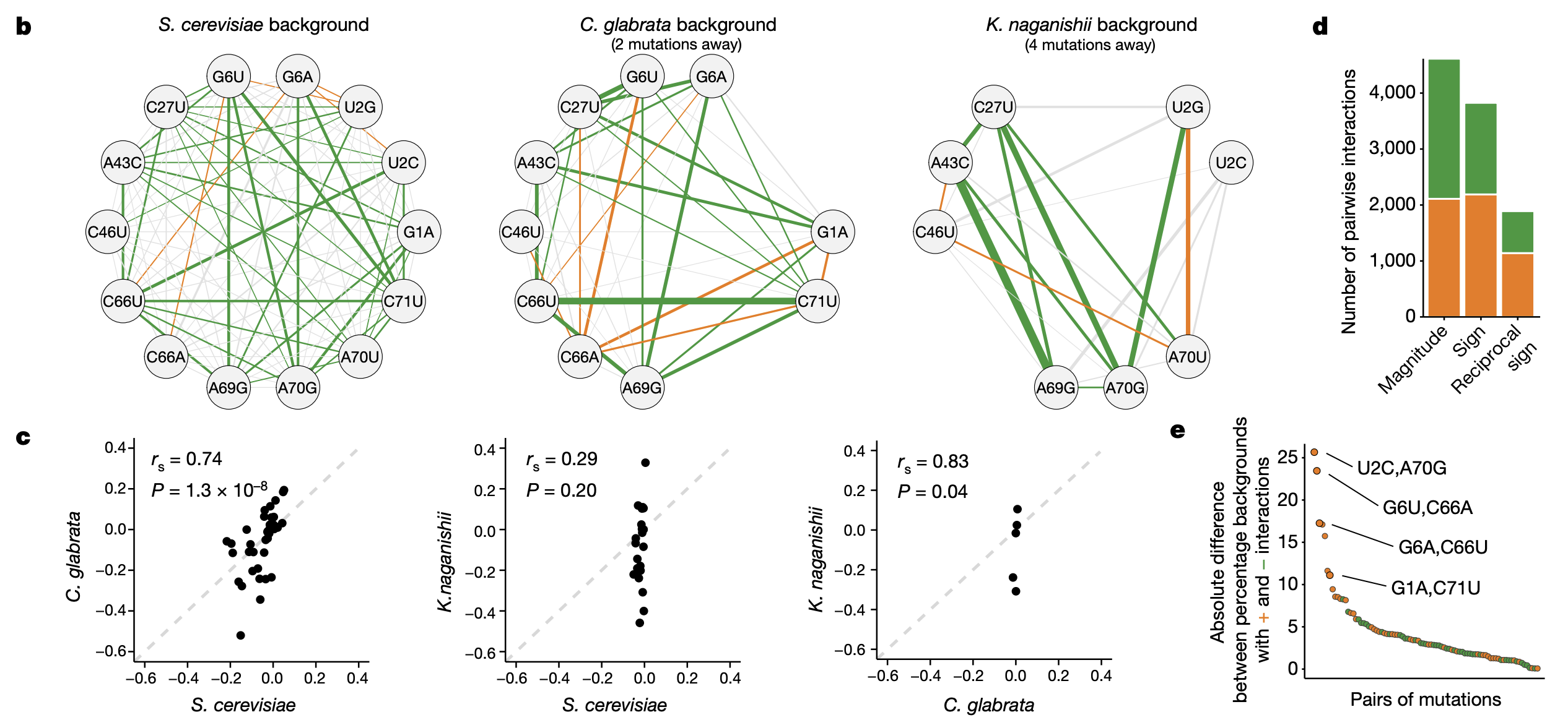
3b: Pairwise epistatic effects in 3 different yeast species. Edge color indicates sign and thickness indicates significance.
3c: Concordance of pairwise epistatic effects between the different species (all shared pairs of mutants between the species are plotted)
3d: Magnitude epistasis: the sign of either mutation does not change in the presence of the other. Sign epistasis: the sign of one mutation has the opposite effect in the presence of the other. Reciprocal sign epistasis: the sign of both mutations have the opposite effect in the presence of the other. Shown here are the number of significant positive (orange) and negative (green) epistatic effects in each category of epistasis.
3e: Difference between number of genotypes with positive vs. negative effects for each pairwise epistatic effect. Higher value = effect is positive in a higher proportion of genotypes (Why did the authors go with this quantity? Isn’t something similar captured by the background-averaged epistatic effect?) Four base pairs that restore Watson-Crick base pairing (WCBP) have some of the most consistently positive pairwise epistatic effects across all background genotypes. WCBP arises from particular locations on the tRNA that loop back and base pair with each other (Fig 1b reproduced below). For these 6? locations, when one variant is mutated, the base pairing is destroyed, but can be restored by another variant.
Extended Data 5d-e
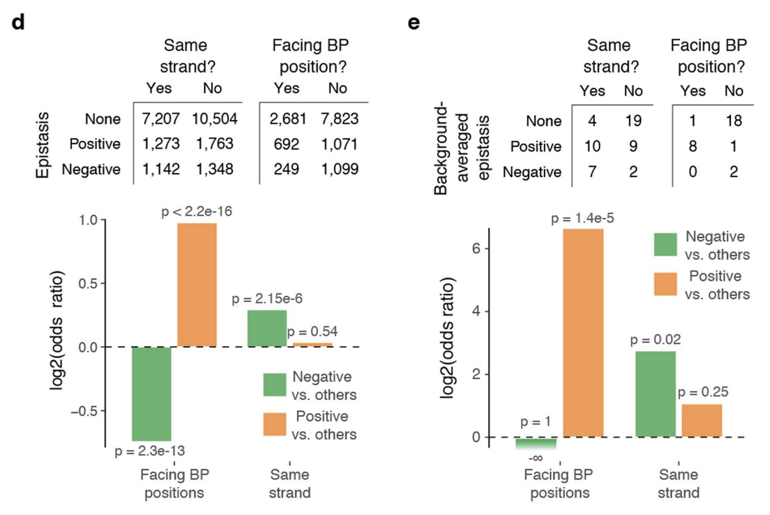
5d: Number of positive and negative pairwise epistatic terms across all genetic backgrounds for base pairs within the acceptor stem, a.k.a. the part at the top of the tRNA that attaches to the amino acid (see above figure). Double mutants for base pairs facing each other are depleted for negative pairwise effects and enriched for positive pairwise effects relative to base pairs not facing each other (bottom left barplot), while double mutants on the same strand are enriched for negative pairwise effects relative to double mutants on different strands (bottom right barplot).
5e: Same plot as 5d but showing background-averaged epistatic terms instead of all epistatic terms.
Extended Data 5f
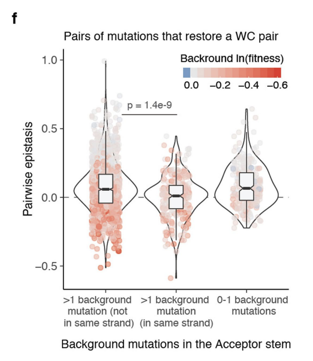
5f: Epistatic effects of double mutants that restore WCBP, stratified by the number of background mutations on the same strand or different strands (What is the mutation relative to? C. cerevisiae?). Interestingly, the effects tend to be more negative when there are multiple mutations on the same strand vs. opposite strands (middle boxplot vs. left boxplot). In other words, having multiple other mutations on the same strand hinder the restoration of WCBP from restoring the fitness of the sample.
Figure 4a-c
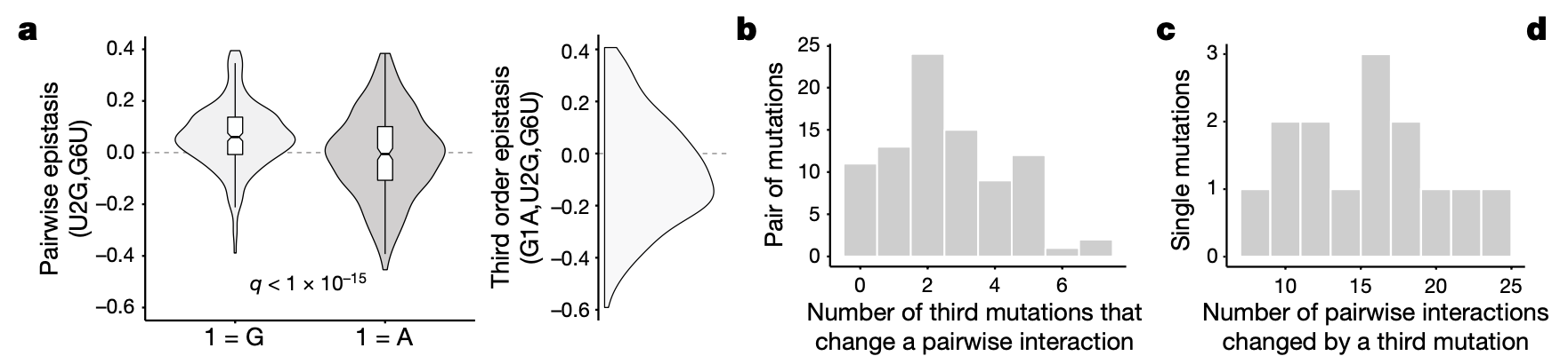
4a: Example of third order epistasis. Shown is the distribution of the pairwise effect of a given mutant pair (U2G,G6U) across all background genotypes with and without an additional mutant (G1A). The density plot on the right is the distribution of third order effects across all background genotypes.
4b: Histogram of mutant pairs that participate in a significant background-averaged third order effect. X-axis: number of distinct third order effects. Most mutant pairs participate in at least one third order effect.
4c: Histogram of individual mutants that participate in a significant background-averaged third order effect. X-axis: number of distinct third order effects. All individual mutants participate in at least 8 third order effects.
Extended Data 7c-d
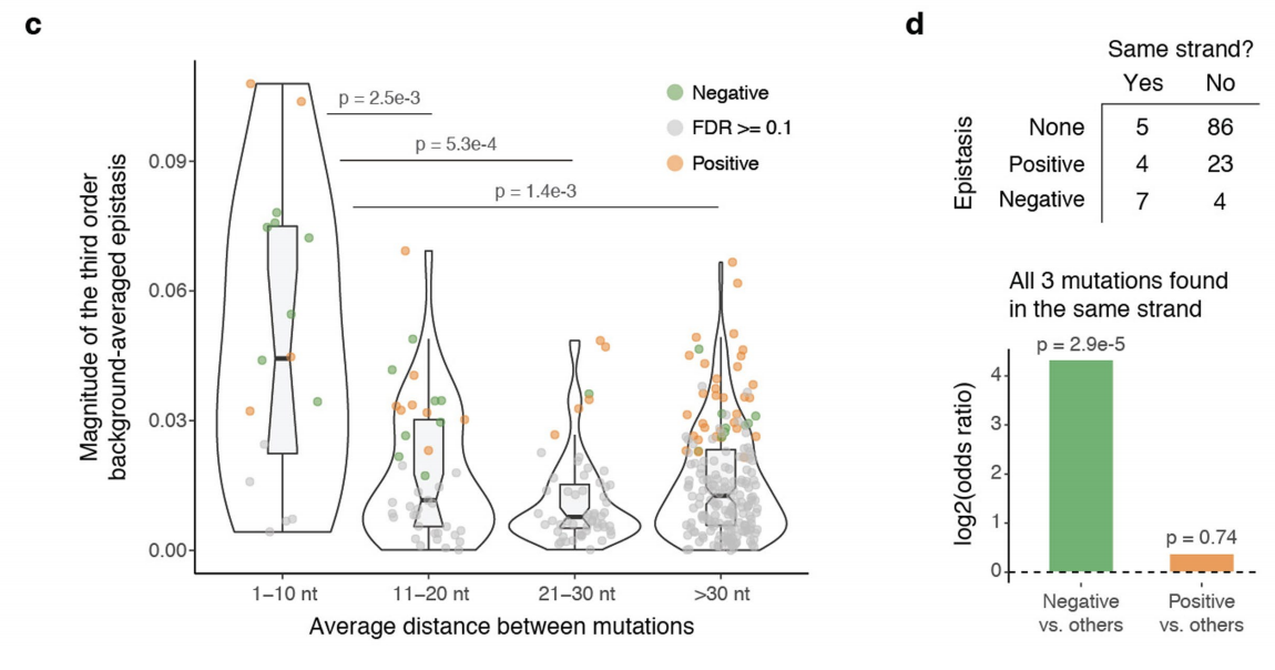
7c: 3rd order effects are larger in magnitude when mutants are physically closer together. Y-axis: magnitude of background-averaged 3rd order effect. X-axis: Average distance between mutants (in nucleotides).
7d: 3rd order effects are more likely to be negative when all 3 mutations are on the same strand.
Figure 4d
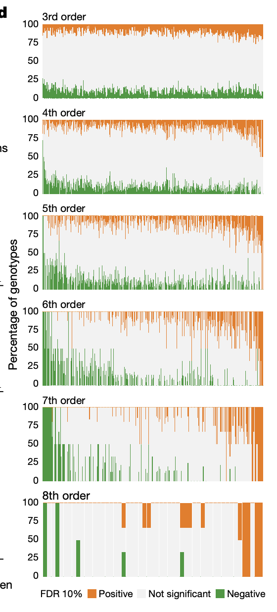
4d: x-axis: all nth order effects. Each “column” represents a given nth order effect. y-axis: Proportion of background genotypes in which the given nth order effect is positive or negative.
Figure 4e-f
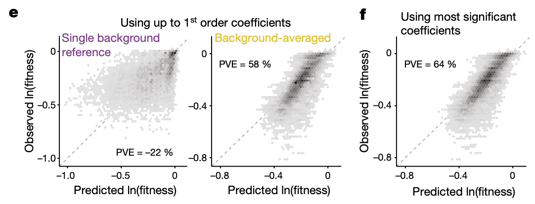
4e: Prediction of log(fitness) from 1st order coefficients from either a single reference (which one, or is it all possible backgrounds?) or from background-averaged 1st order coefficients. _I’m assuming the author meant PVE = 22% on the left? How can it be negative? _
4f: Prediction of log(fitness) from only significant background-averaged epistatic terms (20 out of 256, \(256 = 2^8\) comes from the downsampling the genotypes for cross-validation which prevents 7th and 8th order coefficients from being computed). The fact that the phenotypes can be predicted well from a small number of epistatic terms suggests that they are sparse.
Figure 4g
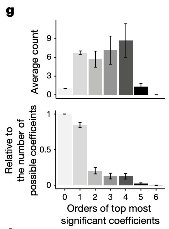
4g: Histogram of number of significant terms as a function of order. Top: absolute number of significant terms. Bottom: number of significant terms relative to the number of possible terms at each order.