Authors: Shiquan Sun, Jiaqiang Zhu, and Xiang Zhou
Synopsis
This paper proposes a new method to determine whether given spatial gene expression data, there is any relationship between expression level and spatial coordinates. The method is built upon a generalized linear spatial model (GLSM) and directly models count data unlike other methods (which transform count data before analysis), leading to better type 1 error control and higher power. It is also fully parametric and much more computationally efficient than non-parametric methods.
Summary
Figure 1A
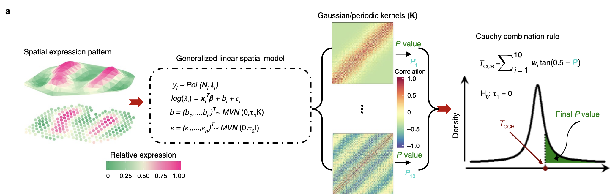
Overview of method. Spatial count data is modeled using generalized linear spatial model (GLSM), where the spatial process is captured by a random effect. The GLSM has been previously used for interpolation and prediction of spatial data but is extended to hypothesis testing in the study. “Spatial coordinate” can be 3-D or include time as a dimension.
In the figure, \(y_i\) represents the expression at a particular spatial coordinate for sample \(i\), \(N_i\) is a scale factor (used to normalize total expression of each coordinate across samples to be the same), and \(\lambda_i\) is a Poisson rate parameter that depends on underlying gene expression level as well as sample \(i\). \(\log(\lambda)\) follows a linear model with \(x\) representing a vector of covariates, \(\epsilon\) representing residual error, and \(b\) representing a random effect capturing spatial correlation patterns. \(b\) for each spatial coordinate is drawn from a 0-mean multivariate normal with covariance \(K\), which has a kernel function of the spatial locations.
The spatial kernel function can be specified arbitrarily in order to capture specific spatial patterns. For example, a Gaussian kernel is useful for clustered expression patterns, while a periodic kernel useful for oscillating expression pattern. The authors ended up picking 10 kernels (5 periodic kernels with different periodicity parameters and 5 Gaussian kernels with different smoothness parameters), then aggregate across all kernels.
The null hypothesis is that \(\tau_1 = 0 \). P-values were computed for each kernel using the Satterthwaite method, then aggregated across 10 kernels using the Cauchy combination rule.