Authors: Iain M. Johnstone and Debashis Paul
Synopsis
This paper provides a review of the properties of eigenvalues and eigenvectors of the random covariance matrices in which the data is “high dimensional” (or the number of features is comparable to the number of samples). It turns out that the eigenvalues of such matrices exhibit some really interesting properties. This information is pertinent for answering questions like: “which eigenvectors/eigenvalues of a matrix are significant?” or “what proportion of variance in a matrix can be explained by low-rank signal vs. independent noise?”
Summary
Background
When performing PCA, we start with a \(p \times n\) matrix \(X\), where \(n\) is the number of samples and \(p\) is the number of features. We then find the eigenvalues and eigenvectors of the \(p \times p \) sample covariance matrix \(\frac{1}{n} X X^T \). Although PCA is simply a procedure applied to a matrix of fixed values, it can also be conceptualized in terms of random matrices, in which each sample is drawn from a multivariate distribution with some mean vector and covariance matrix.
As \(n\) goes to infinity and \(p\) is fixed, the sample covariance matrix will converge to the population covariance matrix (a.k.a \(E[XX^T]\)), and the sample eigenvalues will also converge to the population eigenvalues. However, what happens if \(n\) and \(p\) _both _go to infinity and the ratio \(\frac{p}{n}\) stays constant? What will the eigenvalues of the sample covariance matrix look like? This is the boundary case in which the paper focuses on.
Figure 2
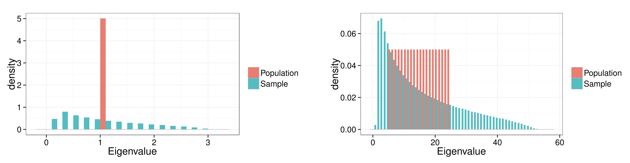
This figure illustrates the phenomenon known as “eigenvalue spreading,” in which sample eigenvalues are more spread out than population eigenvalues. Both figures denote a scenario in which the matrix has \(p\) = 100 features. On the left, all 100 eigenvalues of the population covariance matrix are equal to 1, while the eigenvalues of the sample covariance matrix (where \(n\) = 200) are spread out. The same phenomenon is observed when the eigenvalues of the population covariance matrix are spread evenly between 5 and 25 (on the right).
Figure 3
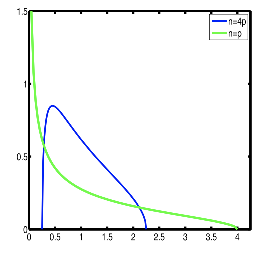
Given a random matrix (features mean centered and variance standardized, samples iid), when \(n\) and \(p\) go to infinity and their ratio stays constant, the distribution of eigenvalues of the sample covariance matrix will converge to a Marchenko-Pastur distribution (which depends only on the ratio between \(n\) and \(p\)). This figures shows what this distribution looks like for two values \(\frac{n}{p} = 1\) and \(\frac{n}{p} = 4\).
Figure 4
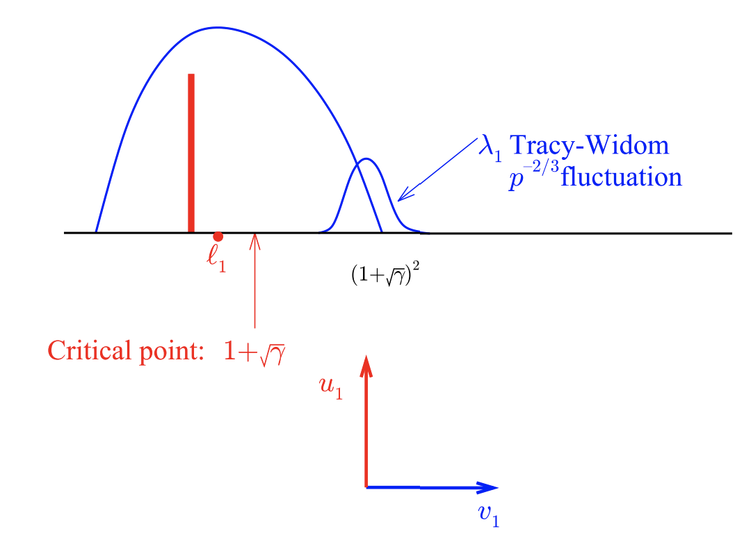
This figure describes the distribution of the largest eigenvalue in random covariance matrices. A very interesting fact is that even if the population covariance matrix has eigenvalues that are larger than 1, if these eigenvalues are smaller than some critical point indicated in the figure, then the distribution of sample eigenvalues will be indistinguishable from that arising from a population covariance matrix in which all eigenvalues are equal to 1.
First, the way we model this is through the “spiked covariance” model, which is a way to model noise on top of low-rank structure. The model involves a “base” covariance matrix \(\Sigma_0\) and a low-rank perturbation:
\[ \Sigma = \Sigma_0 + \sum_k^K h_k \mathbf{u}_k \mathbf{u}_k^T \]
In the simplest case, \(\Sigma_0\) is the identity matrix, while \(h_k\) and \(\mathbf{u}_k\) are the eigenvalues and eigenvectors respectively of some low-rank structure in the covariance matrix. This model is called the “spiked” covariance model because it results in a population eigenvalue distribution with many points at 1 (corresponding to noise) and spikes at each \(h_k\) (corresponding to signal). This can also be conceptualized in terms of the probabilistic PCA model \(\mathbf{x = Wz + e}\), where \(\mathbf{x}\) is our sample, \(\mathbf{W}\) are all the eigenvectors of the sample covariance matrix, \(\mathbf{z}\) are the projected points in PC space (assumed to be randomly drawn from \(N(\mathbf{0}, \mathbf{I})\)), and \(\mathbf{e}\) is isotropic noise (drawn from \(N(\mathbf{0}, \mathbf{I})\)). The covariance matrix of \(\mathbf{x}\) is defined as \(\mathbf{W W}^T + \mathbf{I}\).
Continuing on: let \(l_1\) represent an eigenvalue of our matrix greater than 1, with the remaining eigenvalues equal to 1. If \(l_1\) is smaller than \(1 + \sqrt{\gamma}\) (where \(\gamma\) is \(\frac{p}{n}\)), then the distribution of eigenvalues will be exactly the same as if \(l_1 = 1\) (a.k.a. it will look as if the matrix has no low-rank structure at all. This fact is pretty cool). Moreover, the corresponding eigenvector for \(l_1\) will be completely uncorrelated with the true eigenvector. The top eigenvalue will be distributed according to a Tracy-Widom distribution around the value \((1 + \sqrt{\gamma})^2\).
Figure 5
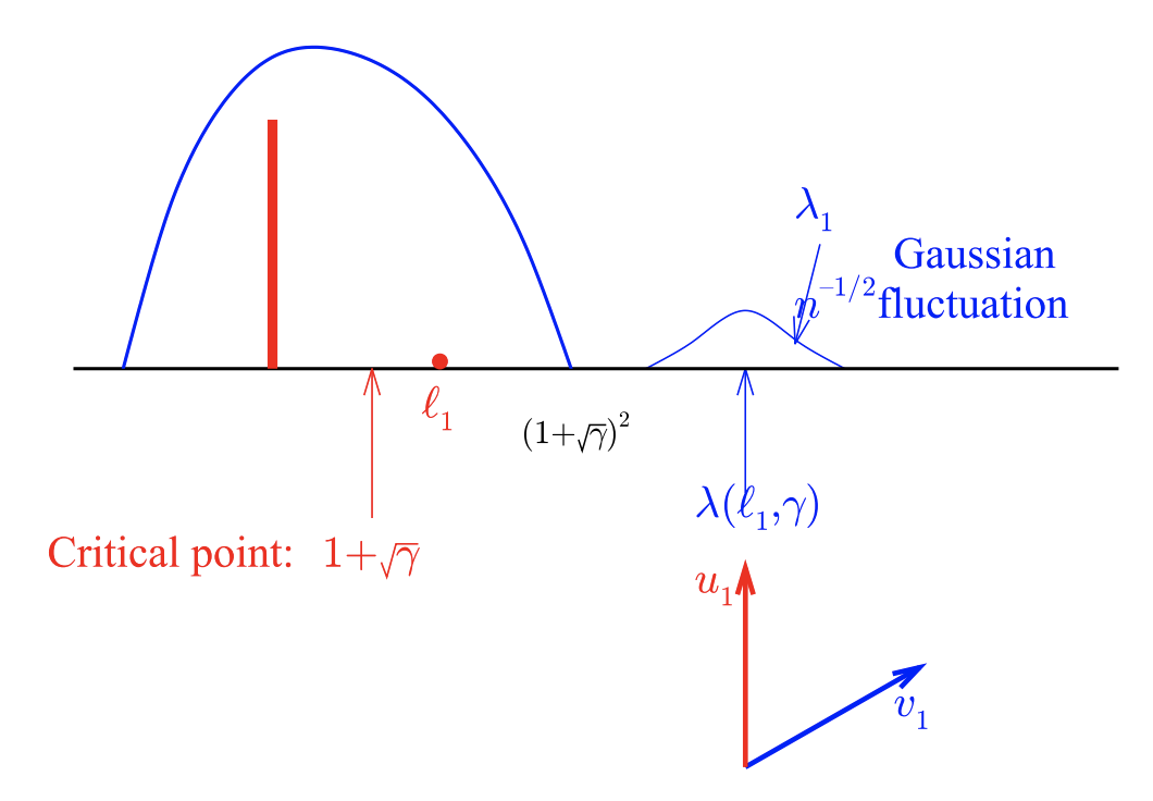
This figure describes the scenario in which the population covariance matrix has eigenvalues that are larger than the critical point. If \(l_1\) is greater than \(1 + \sqrt{\gamma}\), then the top eigenvalue will now be distributed according to a Gaussian distribution while being significantly upwardly biased relative to \(l_1\) (interesting!). Meanwhile, the corresponding eigenvector will now be correlated with the true eigenvector, where the degree of correlation will depend on \(l_1\) and \(\gamma\):
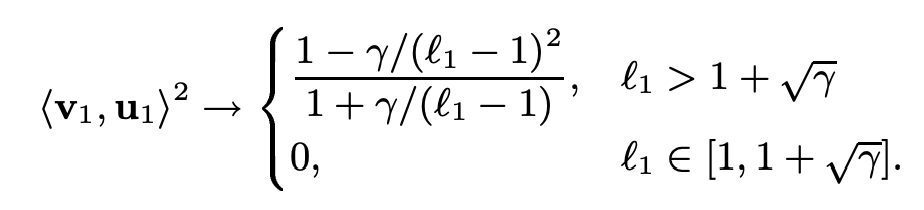
Figure 6
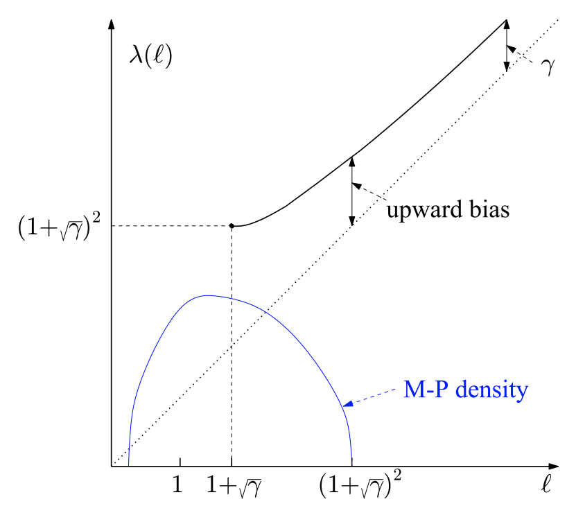
This figure shows the relationship between upward bias of \(\lambda(l_1)\) (a.k.a. the sample value of \(l_1\)) relative to its population value. The upward bias will converge to \(\gamma\) as \(l_1\) increases. More precisely, we have the following relationship between \(\lambda(l_1)\) and \(l_1\):
\[ \lambda(l_1) - l_1 = \gamma \frac{l_1}{l_1 - 1} \]