This blog post is meant to accompany my paper “Quantifying genetic effects on disease mediated by assayed gene expression levels” (Yao et al. 2020 Nature Genetics), in which we introduced a method called “mediated expression score regression” (MESC) to estimate a quantity “heritability mediated by gene expression levels.” I had originally meant to write it when the paper came out, but better late then never I guess. The paper is unfortunately pretty dense and probably not very accessible to readers not in the field of statistical genetics, so I’m hoping to provide a non-technical overview of the paper, in which I describe the background, motivation, method, and assumptions. I’m assuming that you already have a working knowledge of what GWAS and heritability are. If you’re fuzzy about heritability, you can read my other blog post about it. I also included a glossary that defines all the lingo used in this post (terms such as “heritability enrichment” and “Mendelian randomization”), though I tried my best to define everything in the text. Note that I’ll use the terms “trait” and “disease” interchangeably, as well as “SNP” and “variant.” For a more general overview of the paper aimed at a non-technical audience, see here.
Table of contents
- Background
- Defining disease heritability mediated by gene expression levels
- Estimating disease heritability mediated by gene expression levels
- Model assumptions
- A brief comment on gene set analyses
- Miscellaneous points
- Glossary
Background
A while ago, researchers realized that most of the GWAS hits they found fell into non-coding parts of the genome.
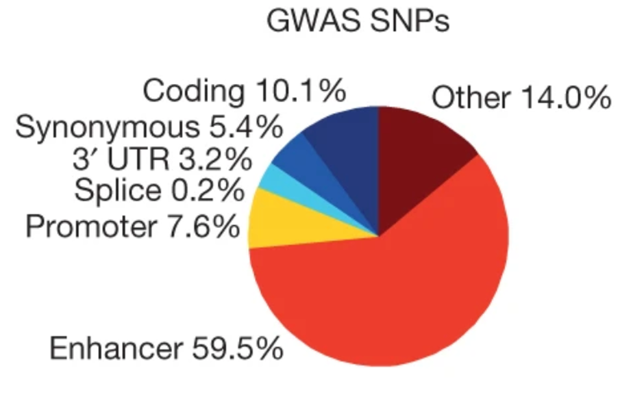
If you think about how a non-coding SNP might exert its effect on a trait, the first thing that comes to mind is via gene regulation (in other words, altering gene expression levels). This was the motivation behind a series of massive efforts to measure expression quantitative trait loci (eQTLs). The most salient of these efforts has been the Genotype-Tissue Expression (GTEx) Consortium, which measured expression levels in ~50 tissues for around ~500 individuals. From these studies, many thousands of significant eQTLs covering almost all genes across many tissues have been detected.
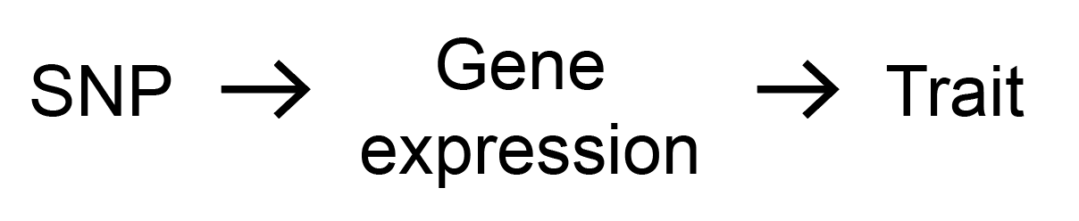
Now, what do we do with these eQTLs after measuring them? In particular, how do we integrate them with GWAS hits to tell us something about how the GWAS hits are acting on the phenotype? Many approaches have been developed to do this on an individual gene level, which include “colocalization tests” and “transcriptome-wide association studies” (TWAS). Long story short, these methods basically look for genes with some sort of “overlap” between their eQTLs and GWAS hits. If a SNP is both a GWAS hit and an eQTL for a given gene, then we would be inclined to think that this gene is somehow important in the SNP’s mechanism of action on the trait. In particular, we would like to think that the SNP’s effect on the trait is mediated through that gene’s expression as illustrated below.
Although this mediation scenario is what we want to see, there are in fact other less desirable scenarios that are indistinguishable from mediation to colocalization/TWAS. I will discuss some of these scenarios in a bit.
The individual-gene methods are interesting and useful ways to prioritize disease-relevant genes. However, perhaps we’d like to take a step back and understand the overall importance of gene expression in “explaining” a phenotype. Understanding this importance can guide our individual gene analyses and give us an overall idea of how disease-relevant our gene expression measurements are.
With regard to this aim, there had already been some work done before our paper came out. Hormozdiari et al. (2018) looked at the overall heritability enrichment of SNPs that we deem to be eQTLs, finding that fine-mapped eQTLs as a whole are enriched for disease heritability. In addition, Chun et al. (2017) looked to see what proportion of significant GWAS hits for autoimmune disease “colocalize” with immune cell eQTLs, finding that only 25% of GWAS hits do so. These results give us an idea of how relevant eQTLs as a whole are to disease. We can see the eQTLs are more disease-relevant than random SNPs (as evidenced by their heritability enrichment), but there are signs that some GWAS hits do not overlap with eQTLs, suggesting that perhaps our eQTL data is not capturing disease mechanisms as well as we would hope.
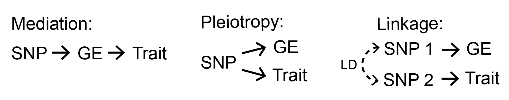
However, there are some important drawbacks to all the previous approaches I’ve described so far. In particular, these approaches cannot distinguish “mediation” (our desired scenario) from other causality scenarios. Two of these scenarios include “pleiotropy” (in which the same SNP affects gene expression and disease independently of each other) and “linkage” (in which two SNPs separately affect gene expression and disease but are in LD with each other). The colocalization-based methods try to rule out linkage as an explanation for overlap between eQTLs and GWAS hits, but none of the methods can (nor do they attempt to) distinguish pleiotropy from mediation.
This brings us to our paper. In my opinion, the most direct way to understand how “important” eQTLs are to disease is via some sort of quantification of mediation, since mediation is how we tend to conceptualize the involvement of gene expression in disease. How do we measure mediation? We decided to do this by quantifying the proportion of disease heritability that is mediated by gene expression levels. In the process of doing this, we’ll try to distinguish mediation from pleiotropy/linkage. First, I’ll go into the definition of the quantity we aim to estimate.
Defining “disease heritability mediated by gene expression levels”
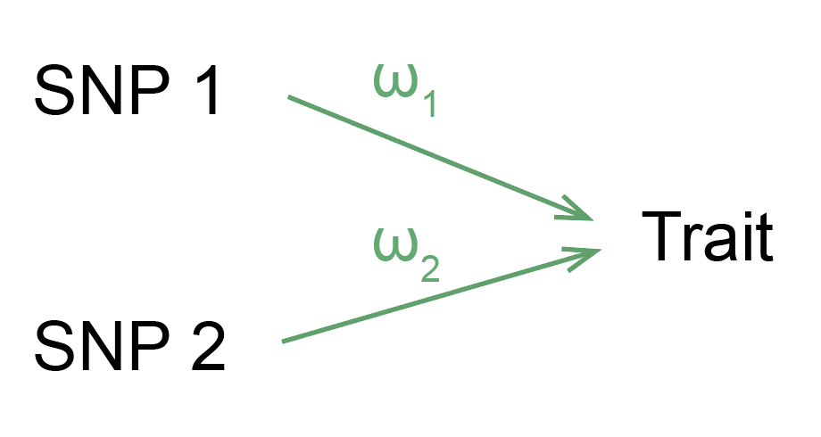
Heritability is a natural way to think about the total effect of genetics on a trait. We can imagine that each SNP exerts some causal effect on the disease, which we’ll call \( \omega_k \) for SNP \( k \) (usually people use \( \beta \) to refer to this quantity, but I ended up using \( \beta \) for eQTL effect sizes in the paper instead - my bad.)
Now, we can instead think about a model in which each SNP’s effect on disease is mediated through the expression of one or more genes.
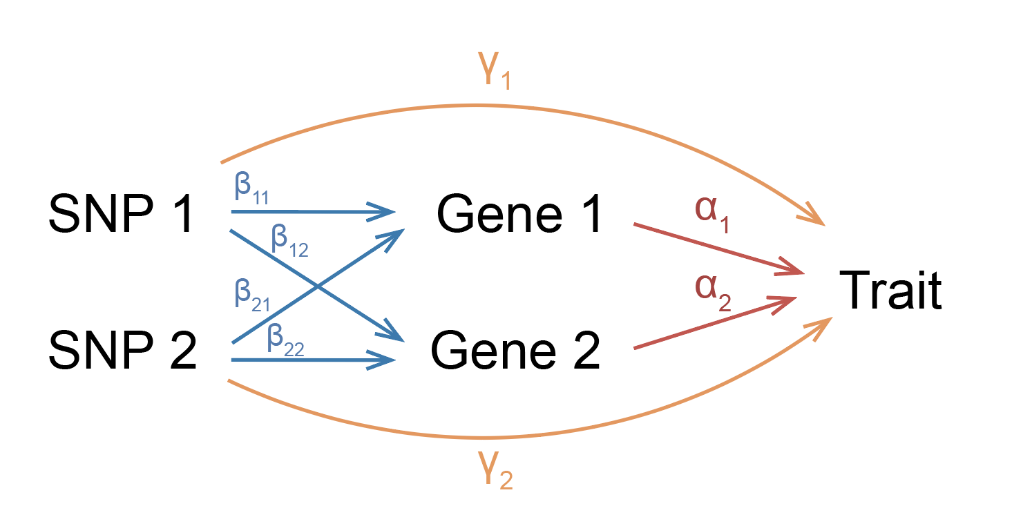
Note that in our model, each SNP effect size has a mediated component and a non-mediated component. The mediated component can be broken down into the product of eQTL effect sizes and gene effect sizes on trait.
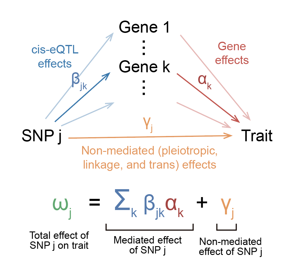
In this model, we can feel free to interpret these effect sizes in the most intuitive way possible: \(\beta_{jk}\) represents the change in expression of gene \(k\) in individuals carrying an allele of SNP \(j\), \(\alpha_k\) is the change in trait per unit change in expression of gene \(k\), and \(\gamma_j\) is the extra change in the trait in individuals carrying an allele of SNP \(j\) that doesn’t go through expression. Because we don’t want to weigh highly expressed or variable genes more than others, we’ll scale gene expression to have the same mean and variance across all genes. Thus, you can think of eQTL effect sizes in terms of expression change proportional to overall expression and variance of the gene.
How do we quantify overall mediation? Well, one way to do it would be to just take all the mediated parts of each effect size and sum them up. Because effect sizes can be positive or negative, we’ll square everything. We end up with a quantity that I’ll call \(h_{med}^2\):
\[h_{med}^2 = \sum_{j} \sum_{k} \beta_{jk}^2 \alpha_k^2 \]
Finally, we can divide this quantity by the total SNP effect on disease \( \sum_j \omega_j^2 \) to get the proportion of total SNP effect on disease mediated by gene expression.
\[\frac{h_{med}^2}{h_g^2} = \frac{\sum_{j} \sum_{k} \beta_{jk}^2 \alpha_k^2}{\sum_j \omega_j^2} \]
We have now defined the quantity we want to estimate (well, not exactly; see below.)
Technical point 1: In practice, we don’t quite estimate \(h_{med}^2\) as defined above. We like to operate in units of heritability (which are comparable across different traits in different populations). When operating in units of heritability, each SNP effect size is scaled by the variance of the SNP’s minor allele count, which in turn depends on the SNP’s minor allele frequency (MAF) in the population. In other words, SNPs contribute to heritability proportional to both their per-allele effect size (what we intuitively think of as their effect size in an individual) as well as their MAF, which causes common variants to contribute more to heritability than rare variants. Working with scaled effect sizes enables us to write \(h_g^2 = \sum_j \omega_j^2 \), without having to think about the variance of individual SNP counts. Scaling effect sizes by MAF may lead us to change our interpretation of these effect sizes, but I’ll posit that we don’t have to change our interpretation that much (since in our study we look at only common variants, for which there isn’t a strong relationship between per-allele effect size and MAF). If this point is confusing, it may be helpful to read my other blog post on heritability.
Technical point 2: This point is extra technical but I’ll talk about it anyway for completeness. Whenever I talk about “heritability,” I will be referring specifically to SNP heritability \(h_g^2\). Here, the set of SNPs includes all common SNPs (a.k.a. MAF \(\geq\) 0.05) in Europeans from the 1000 Genomes reference panel. When thinking in terms of SNP heritability, it’s not quite appropriate to think of \(\omega_j\) or \(\beta_{jk}\) as representing the causal effect size of SNP \(j\). It will actually represent this causal effect size in addition to tagging effects of any SNPs in LD with SNP \(j\) that are not included in the set of common SNPs being studied. However, in practice, common SNPs found in 1000 Genomes Europeans include almost all common SNPs in any European population, and common variants do not really tag rare variants, so we can interpret \(\omega_j\) or \(\beta_{jk}\) as basically the causal effect size of just SNP \(j\).
Ok, so we have our quantity that we want to estimate: \(h_{med}^2\). Well, not quite. I need to give one more definition of a quantity known as heritability mediated by assayed gene expression, which is what we end up actually estimating in practice. In the above model, we assume that gene expression is taken in the causal cell types and/or cellular contexts for a given disease. As you can imagine, gene expression can vary greatly across different cell types/contexts, but we only think of mediation as occurring through gene expression levels in these causal cell types for disease (for example, neurons for schizophrenia, immune cells for lupus, etc.). Thus, in order to actually estimate \(h_{med}^2\) when gene expression is taken in the causal cell types/contexts for the disease (we’ll call this quantity \(h_{med;causal}^2\)), we would need to be able to measure eQTLs in all these cell types/contexts. This data does not exist at the moment. In fact, for many diseases we don’t even know what the exact causal cell types/contexts are.
In practice, the best we have is the set of 50 or so bulk tissues from GTEx, which likely capture expression some causal cell types for a given disease but not all. How do we make use of this data? We can define an alternative version of \(h_{med}^2\) that we’ll call \(h_{med;assayed}^2\), which assumes that expression measurements are coming from a given assayed tissue rather than the causal cell types/contexts for the disease. If you think about it, it doesn’t really make sense to think of SNP effects on disease as being mediated through the expression of a gene in an irrelevant tissue. However, expression in different tissues is actually quite similar overall, as reflected in the fact that eQTL effect sizes are quite correlated with each other across different tissues (see e.g. Liu et al. 2017). Thus, even if a tissue is irrelevant to a disease, it will “tag” the expression of truly causal cell types and contexts.
Now for the actual definition of \(h_{med;assayed}^2\). The definition is \(h_{med;assayed}^2(T) = r_g^2(T) h_{med;causal}^2\). We include the \((T)\) symbol because this quantity depends on the set of assayed tissue(s) (which we’ll call \(T\)) from which we measured eQTLs. \(r_g^2(T)\) is the squared genetic correlation between expression in \(T\) and expression in the causal cell types/contexts for the disease (a.k.a the squared correlation in eQTL effect sizes), averaged across all genes. \(r_g^2(T)\) gives us a measure of how similar our assayed tissue is to the unknown or unmeasured causal tissue/contexts. THIS is the final quantity that gets estimated in practice. You might think that this definition comes out of nowhere, but we have derivations and simulations that show that when MESC estimates \(h_{med}^2\) using eQTL measurements from an arbitrary set of tissues \(T\), this is the exact quantity that comes out (assuming that all other assumptions are satisfied). Also note that we cannot separate the terms \(r_g^2(T)\) and \(h_{med;causal}^2\); we can only estimate their product.
How do we interpret \(h_{med;assayed}^2(T)\)? \(r_g^2(T)\) has to be less than or equal to 1, so \(h_{med;assayed}^2(T) \leq h_{med;causal}^2\). If our assayed tissue(s) is exactly the causal tissue(s) for the disease, then we’ll have \(h_{med;assayed}^2(T) = h_{med;causal}^2\). We can think of \(h_{med;assayed}^2(T)\) as reflecting two things: the true amount of mediation occurring in the causal cell types/contexts for the disease (as captured by \(h_{med;causal}^2\)), and how well the assayed tissue “tags” the causal tissue (as captured by \(r_g^2(T)\)). Although it would be interesting to know what \(h_{med;causal}^2\) is, at the moment we have no way of estimating it. Moreover, I would argue that \(h_{med;assayed}^2(T)\) is as important to know as \(h_{med;causal}^2\), since it reflects how “important” our assayed expression measurements are to disease. Indeed, for all eQTL-related analyses, people only have access to these assayed expression measurements rather than expression in causal cell types/contexts. For brevity, I will refer to \(h_{med;assayed}^2(T)\) as just \(h_{med}^2\) for the remainder of the post, but keep in mind that all results will reflect \(h_{med;assayed}^2(T)\) rather than \(h_{med;causal}^2\).
Finally done with definitions. Now, for the actual hard part: estimating \(h_{med}^2\). In the process of estimating this quantity, we will have to distinguish mediation from the other undesirable scenarios such as pleiotropy and linkage. Let’s go into how we do this.
Estimating disease heritability mediated by gene expression levels
People have already thought about ways to try to distinguish pleiotropy from mediation, in particular under the umbrella of Mendelian randomization (MR) methods. There are many different types of MR, which all come with their own bag of assumptions and pros/cons. The core idea behind MR (when applied to gene expression) is that if a gene’s expression is truly mediating genetic effects on disease, then SNP effects on the gene should be proportional to SNP effects on the disease.
This is the core idea behind MESC as well (and is also closely related to TWAS/genetic correlation), so I think it’s worth driving home. Let’s walk through an example. For simplicity, let’s assume that LD doesn’t exist, so we can measure causal rather than marginal SNP effect sizes. Let’s also assume for the moment that our eQTL measurements are taken in the causal cell types/contexts for the disease (rather than from assayed tissues). These two things are obviously not true in practice, but they don’t really change the following exposition. Either way, we’ll talk about how to handle these things later.
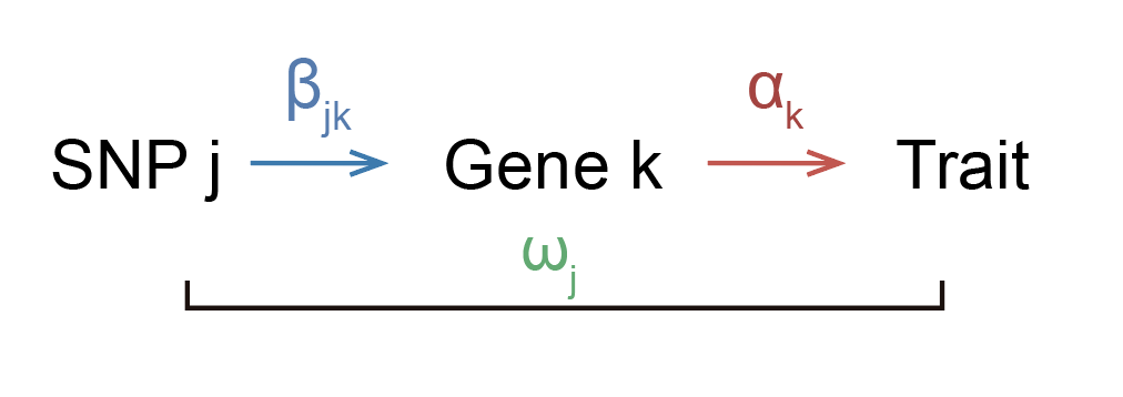
Suppose that we know in reality that increasing expression of gene \(k\) by 1 (in some units) will increase trait by \(\alpha_k\) (in some units). Now, suppose that SNP \(j\) increases the expression of gene \(k\) by \(\beta_{jk}\). If the SNP does not affect anything other than the expression of gene \(k\), then the SNP should also increase the trait by \(\beta_{jk} \alpha_k\). Note that we cannot measure \(\alpha_k\), but we can measure \(\beta_{jk}\) and \(\omega_j\) from an eQTL study and GWAS respectively. We can thus divide \(\omega_j\) by \(\beta_{jk}\) to get an estimate of \(\alpha_k\).
You might think that it’s unrealistic that the entire effect of the SNP on trait is going through the gene, and you’d probably be correct. Perhaps a more realistic model would look like this:
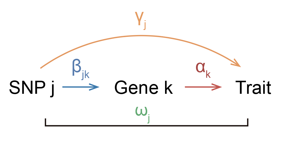
where the SNP has some effect on the trait that isn’t going through the gene. Ok, so how do we estimate \(\alpha_k\) now? It’s tricky if we just look at one SNP, but if we have multiple SNPs that affect the gene, then we have a way to approach this problem. The idea is that the mediated component of each SNP effect size should be exactly equal to \(\beta_{jk} \alpha_k\) across SNPs.
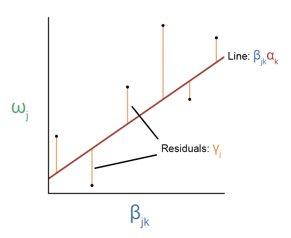
Here, each point represents a SNP. Because we have multiple SNPs affecting the same gene, we can regress \(\omega_j\) on \(\beta_{jk} \) to estimate the slope of the line, which should equal \(\alpha_k\).
There are of course several assumptions we need to make in order for this procedure to give us an accurate estimate of \(\alpha_k\). One assumption is known in MR literature as the InSIDE (INstrument Strength Independent of Direct Effect) assumption, which says that \(\gamma_j\) cannot be correlated with \(\beta_{jk}\). Another assumption is that we have no noise in our estimates of \(\beta_{jk}\), otherwise our slope estimate will be downwardly biased due to regression attenuation. Third, there is the assumption that the mediated component of these SNP effects is a linear function of \(\beta_{jk}\). I mention these assumptions because they all have direct analogs in the MESC framework.
Onto MESC. Recall that our goal is to estimate the quantity \(h_{med}^2\) (or \(\sum_{j} \sum_{k} \beta_{jk}^2 \alpha_k^2 \)). One way to do this would be to separately estimate \(\beta_{jk} \alpha_k\) for each gene \(k\) using something similar to the approach illustrated above, then square this quantity and sum across genes to get \(h_{med}^2\). It turns out this approach is challenging because \(\beta_{jk} \alpha_k\) estimates for individual genes can be extremely noisy, and in order to estimate the standard error of \(h_{med}^2\) we would need to know the standard errors and covariance structure of all individual \(\beta_{jk}^2 \alpha_k^2\) terms. Instead, we take a different approach. First, we rewrite \(\sum_{j} \sum_{k} \beta_{jk}^2 \alpha_k^2 \) as \(GE[\sum_j \beta_j^2]E[\alpha^2]\), where the expectation is taken over genes and \(G\) is the total number of genes. Note that in order to write this, we need to assume that \(\beta\) is independent of \(\alpha\) (I’ll discuss all the assumptions in a bit). Also note that \(E[\sum_j \beta_j^2]\) is the average gene expression heritability across genes. Now, we can estimate \(E[\alpha^2]\) using the following regression:

How is this regression procedure different from the one above? For one, we’ve squared everything, which is why the residuals are all positive and are reflected in an intercept term. In addition, instead of regressing \(\omega_j\) on \(\beta_{jk}\) for a single gene, we are regressing \(\omega_j^2\) on \(\sum_k \beta_{jk}^2\) (a.k.a. the sum of eQTL effect sizes across all genes). Thus, the regression will include all genes rather than a single gene. Rather than the slope reflecting a single \(\alpha_k\), the slope from this regression will reflect the average \(\alpha_k^2\) across all genes. As you recall, we have rewritten \(h_{med}^2\) as \(GE[\sum_j \beta_j^2]E[\alpha^2]\), so we can plug in \(E[\alpha^2]\) as estimated by this regression. We can estimate \(E[\sum_j \beta_j^2]\) using standard heritability-estimation methods such as GCTA or LD score regression and plug that into the formula as well. That’s basically it! This is what’s going on at the heart of MESC.
As you can imagine, there are several important assumptions we need to make in order for the above regression to work (and in fact the main technical challenges of the paper were figuring out how to deal with violations to these assumptions). I will discuss these assumptions below. However, first I’d like to talk about how we deal with LD. In practice, we don’t actually have access to causal effect sizes \(\omega_j\) or \(\beta_{jk}\); we typically can only estimate marginal effect sizes (which include tagging effects from SNPs in LD with with given SNP). In particular, most publicly available GWAS data only comes in the form of marginal SNP effect sizes. If we simply replace causal effect sizes with marginal effect sizes in the above regression, then our slope estimate will be confounded by LD (since SNPs will tag the effects of other SNPs causing their marginal \(\omega_j\) and \(\beta_{jk}\) estimates to be larger than their causal \(\omega_j\) and \(\beta_{jk}\)).
We can account for this confounding by simply including a covariate corresponding to the total level of LD of the SNP, or more specifically the LD score of the SNP. This is in fact the exact same LD score that goes into the widely-used LD score regression. When including the SNP’s LD score as a covariate, we we are free to regress marginal \(\omega_j\) estimates on marginal \(\beta_{jk}\) estimates, and our slope estimate will equal \(E[\alpha^2]\) as desired (there is a derivation in the supplementary note of the paper that proves this if you’re curious). We need to make some additional assumptions for this to work, but I’ll discuss all assumptions in the next section.
Finally, what happens when \(\beta_{jk}\) comes from an arbitrary assayed tissue rather than the causal tissues/contexts for the disease? If we perform the regression using assayed \(\beta_{jk}\), then we will end up estimating \(h_{med;assayed}^2(T)\) rather than \(h_{med;causal}^2\) (there is again a derivation for this in the supplement). To give some intuition for this, you can think of assayed \(\beta_{jk}\) as adding “noise” into the independent variable of the regression relative to \(\beta_{jk}\) in causal cell types/contexts. This causes the slope estimate to be lower due to regression attenuation. It turns out that the magnitude that this slope decreases is exactly equal to \(r_g^2(T)\).
Model assumptions
In this section, I’ll describe the main assumptions necessary for MESC to give unbiased estimates of \(h_{med}^2\), what scenarios in which they’ll be violated, and how we try to account for these scenarios in which the assumptions are violated.
(1) \(\beta_{jk}^2\) is uncorrelated with \(\alpha_k^2\)
This assumption states that the magnitude of effect of gene on trait is uncorrelated with eQTL magnitude. In other words, genes with large eQTL effect sizes cannot have systematically different effect sizes on disease as genes with small eQTL effect sizes. Does this assumption hold in practice? Almost certainly no. It has previously been shown that genes depleted for SNPs in their coding regions (which we interpret to mean that the genes affect fitness and thus are important, since SNPs affecting those genes are removed from the population) are also depleted for eQTLs (GTEx Consortium 2017). Thus, we can imagine a scenario in which strong eQTLs for genes with large effects on disease affect the fitness of the individual and are thus removed from the population, causing large-effect genes to only have weak eQTLs. In fact, this is precisely what we ended up observing in our paper.
Violations to this assumption will cause the regression to look something like this:
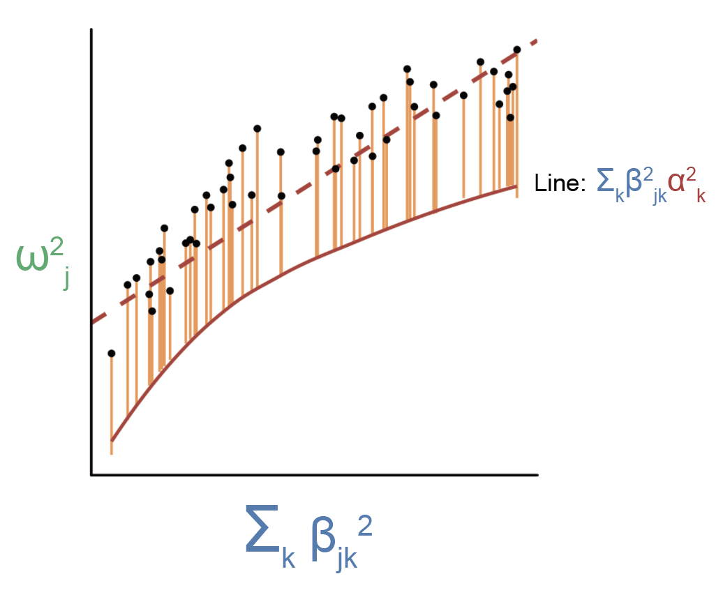
As you can see, there is now a nonlinear relationship between \(\sum_k \beta_{jk}^2\) and \(\sum_k \beta_{jk}^2 \alpha_k^2\) as shown by the red line. The estimated slope from this figure will be less than \(E[\alpha^2]\), since linear regression implicitly weighs point farther away from the origin more than points close to the origin (so the slope will be skewed toward the average \(E[\alpha^2]\) of genes with large effect eQTLs, which we believe to have small \(E[\alpha^2]\)). How do we deal with this issue? One way is to this is to split the regression up over bins of \(\beta_{jk}^2\), in which \(\beta_{jk}^2\) is approximately independent of \(\alpha_k^2\) within the bins. In other words, we can assume that the relationship between \(\sum_k \beta_{jk}^2\) and \(\sum_k \beta_{jk}^2 \alpha_k^2\) is approximately piecewise linear, which enables us to obtain an approximately unbiased estimate of \(E[\alpha^2]\) for each “piece” of the curve. In practice, we ended up splitting all genes into 5 bins, which we showed in simulations was able to adequately correct for biases in \(h_{med}^2\) due to correlations between \(\beta_{jk}^2\) and \(\alpha_k^2\) (the exact number of bins doesn’t really matter so long as there’s at least 5). In practice, it makes a huge difference whether we split genes into bins or not (our average \(\frac{h_{med}^2}{h_g^2}\) estimate across traits goes from 11% to 1% when not splitting genes into bins).
(2) \(\beta_{jk}^2\) is uncorrelated with \(\gamma_j^2\)
This assumption states that the magnitude of non-mediated SNP effect is uncorrelated with eQTL magnitude. In other words, we assume that SNPs with large eQTL effect sizes do not have systematically different non-mediated effect sizes as SNPs with small eQTL effect sizes. Note that this assumption is quite similar to the InSIDE assumption in MR literature. The differences are that the InSIDE assumption (for MR applied to gene expression) applies to only eQTLs for one gene (whereas this assumption applies to eQTLs across all genes), and the InSIDE assumption deals with unsquared effect sizes while this assumption deals squared effect sizes. Does this assumption hold in practice? Unlikely. It’s easy to imagine a scenario in which certain biologically active regions of the genome (for example, promoters) have SNPs with both larger eQTLs and larger non-mediated effect sizes than inactive regions (for example, intergenic regions).
Violations to this assumption will cause the regression to look something like this:
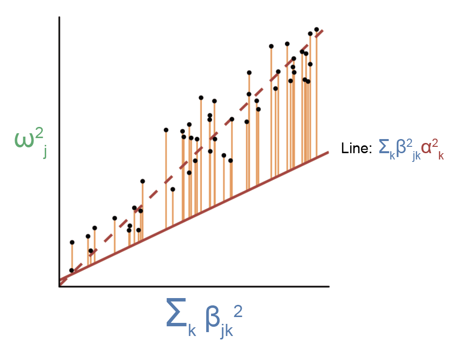
Here, the slope from this regression will be larger than \(E[\alpha^2]\). How do we deal with this issue? In a similar way as the above section, we can split the regression up over bins of \(\beta_{jk}^2\), in which \(\beta_{jk}^2\) is approximately independent of \(\gamma_j^2\) within the bins. For technical reasons, it is challenging for us to directly split SNPs by \(\beta_{jk}^2\). Instead, we assume that the baselineLD model (Finucane et al. 2016, Gazal et al. 2017) (a.k.a. a set of comprehensive SNP categories that includes coding, conserved, promoter, enhancer, histone marks, transcriptions factor bindings sites, etc.) acts as a proxy for \(\beta_{jk}^2\), and we split the regression over the baselineLD model instead. When doing this, we need only assume that \(\beta_{jk}^2\) is uncorrelated with \(\gamma_j^2\) within a given functional SNP category, which is much more likely to be true than when looking at SNPs across different categories. In simulations, we showed that splitting SNPs by the baselineLD model was able to correct for many realistic scenarios in which \(\beta_{jk}^2\) is correlated with \(\gamma_j^2\). In practice, it makes a huge difference whether we split SNPs into categories or not (our average \(\frac{h_{med}^2}{h_g^2}\) estimate across traits goes from 11% to 45% when not splitting SNPs into categories).
To summarize what we have so far, violations to the previous two assumptions in practice require that we slice and dice our regression over both SNP and gene categories in order to ensure approximate independence between \(\beta_{jk}^2\) and both \(\alpha_k^2\) and \(\gamma_j^2\) within each SNP and gene category. Can we guarantee that these things really are approximately independent? No, but we tried hard to make this the case (via simulations and trying out lots of different SNP and gene categories on real data).
(3) LD scores are uncorrelated with both \(\alpha_k^2\) and \(\gamma_j^2\)
This assumption states that the LD score of a SNP (which can be thought of as the total “level of LD” of the SNP) is uncorrelated with \(\alpha_k^2\) and \(\gamma_j^2\). We need to make this assumption in order to work with marginal rather than causal SNP effect sizes. Is this assumption satisfied in practice? Probably not! Previous work has shown that the level of LD of a SNP is correlated with the causal effect size of the SNP on disease (Gazal et al. 2017) (this occurs for complicated reasons that I won’t go into). As a result, it’s not hard to imagine that the level of LD is also correlated with \(\alpha_k^2\) and/or \(\gamma_j^2\). How do we deal with violations to this assumption? Again, by splitting the regression over SNPs (specifically the baselineLD model). The baselineLD model already bins SNPs by both minor allele frequency (which will affect the level of LD of a SNP) and by other metrics of LD, and splitting SNPs by these bins has already been shown to basically account for any relationship between level of LD and SNP effect sizes (Gazal et al. 2017).
(4) There is no sampling noise in eQTL effect size estimates
Of course, there will always be sampling noise in eQTL effect size estimates, so perhaps this should be rephrased as “there is basically no sampling noise in eQTL effect size estimates.” This assumption is an interesting one, as I don’t think that violations to this assumption are necessarily a bad thing. In theory, if we would like to estimate the exact quantity \(r_g^2(T) h_{med;causal}^2\) (where \(r_g^2(T)\) refers to the squared correlation in true effect sizes between assayed vs. causal tissues), we would need an infinite amount of gene expression samples. This again has to do with regression attenuation: if we have any noise in the independent variable (in our case, eQTL effect sizes), then our slope estimate will be downwardly biased.
Of course, we don’t have anywhere near an infinite amount of samples. What we actually end up estimating in practice is a quantity that I’ll call \(\hat r_g^2(T) h_{med;causal}^2\), where \(\hat r_g^2(T)\) is the squared correlation in estimated effect sizes between assayed vs. causal tissues. Any sampling noise in our eQTL effect size estimates will cause \(\hat r_g^2(T) < r_g^2(T)\). In the case of GTEx (particularly when meta-analyzing eQTL effect sizes across tissues, which gives us many thousands of samples), the difference between \(\hat r_g^2(T)\) and \(r_g^2(T)\) is going to be very small, since it’s been shown that our genetic prediction accuracy for cis-eQTL effect sizes is close to optimal for data sets with something like 500 or more samples (in other words, there is very little noise in cis-eQTL effect size estimates for data sets of this size). This fact has been observed in real data (see e.g. Gusev et al. 2016), and we also tested it in simulations in our paper.
However, for data sets much smaller than all GTEx samples (for example, samples in a single GTEx tissue), the difference between \(\hat r_g^2(T)\) and \(r_g^2(T)\) can actually be substantial. Is this bad? Depends on your perspective. If your goal is to estimate the quantity \(r_g^2(T) h_{med;causal}^2\) as accurately as possible (perhaps you want draw some conclusion about the disease-relevance of gene expression in a given tissue without having to think about sample size), then it is a bad thing. If your goal is to get a metric of the disease-relevance of gene expression in a given eQTL data set, then I argue this is not a bad thing and actually reflects the exact metric you want to estimate. Part of an eQTL data set being useful is our ability to accurately estimate eQTLs from that data set. For example, if we have gene expression measurements in the perfect cell type and context for a disease but only 10 samples, then we can’t reliably estimate eQTLs in that data set and thus cannot do any integration of eQTLs with GWAS using that data set (even though in theory the heritability mediated through expression levels in that cell type and context might be large at the limit of infinite samples). Thus, the gene expression measurements from that data set are not going to be very useful (at least from the perspective of eQTLs), and will reflect in a low \(h_{med}^2\) estimate.
(5) Mediated effects of SNPs on disease are linear
This assumption states that the mediated component of SNP effects on disease is linear as a function of eQTL effect size \(\beta_{jk}\). This assumption is quite similar to assumption (1) in the sense that violations to either this assumption or assumption (1) will result in a nonlinear relationship between \(\sum_k \beta_{jk}^2\) and \(\sum_k \beta_{jk}^2 \alpha_k^2\). The difference is that assumption (1) deals with \(\alpha_k^2\) across genes, while this assumptions looks at \(\alpha_k^2\) within individual genes.
There are some reasons why we might expect this assumption to be violated in practice. For example, there may exist compensatory mechanisms that buffer out the phenotypic effects of large changes to a given gene’s expression, but not small changes (see for example Rossi et al. 2015). However, in practice, we can address violations of this assumption in much the same way as violations to assumption (1), in which we assume that that the relationship between \(\sum_k \beta_{jk}^2\) and \(\sum_k \beta_{jk}^2 \alpha_k^2\) is piecewise linear and split the regression accordingly.
There is an additional reason why this assumption is probably not a big deal. Most genes have a single strong cis-eQTL that dominates all others (and in fact this is often the only cis-eQTL that is detectable). This implies that we don’t even have multiple SNPs affecting the same gene for which we might observe nonlinear effects. In our paper, we ended up not really thinking much about this assumption.
A brief comment on gene set analyses
I will briefly talk about using MESC to perform gene set analyses. Although our paper mainly focuses on the heritability mediated by the expression of all genes, it is also of interest to know the heritability mediated by the expression of a particular set of genes (for example, genes in a given pathway). This enables us to do a sort of gene set enrichment analysis in which we identify gene sets with more heritability mediated through their expression than expected given the number of genes in the gene set. There aren’t really any new concepts when estimating heritability mediated by the expression of a given set of genes rather than all genes. You can basically just go through all the previous sections and replace the phrase “all genes” with “genes in the gene set.”
Miscellaneous points
Here, I’ll discuss some miscellaneous points that came up when working on the paper or when discussing the paper with others, which I think are notable enough to write down (as they probably include some questions you might have about the paper).
Role of trans-eQTLs and cis-by-trans eQTLs
Every time I’ve used the word “eQTL” in this blog post so far, I have been referring specifically to cis-eQTLs, which we define to be located within 1 megabase of the gene of interest. Why do we restrict to cis-eQTLs? The main reason is that cis-eQTLs are much stronger and thus easier to estimate than trans-eQTLs. For this reason, cis-eQTLs have been what people have focused on when integrating eQTLs with GWAS. I mentioned previously that our estimates of \(h_{med}^2\) depend on our ability to accurately estimate eQTL effect sizes. For cis-eQTLs, this is possible to do at current sample sizes. For trans-eQTLs, our sample sizes are still much too small (even the largest available eQTL study, eQTLGen (Vosa et al. 2018) which has >30,000 whole blood expression samples, is much too small to accurately predict trans-eQTLs genome-wide.)
Thus, we should think of the quantity that we estimate as the proportion of disease heritability that is mediated through gene expression in cis. Is it possible that there is a substantial heritability mediated through gene expression in trans? Absolutely! In fact, there is nothing stopping us from using the MESC framework to estimate this quantity (where we simply throw in all eQTLs including trans-eQTLs rather than just cis-eQTLs). However, it’s unclear if we’ll get anything meaningful out of this or whether we’ll just be adding noise, even if we have enough expression samples to accurately estimate trans-eQTLs genome-wide (which will be in the 100,000s). The issue is that there are a ton of technical challenges when it comes to accurately estimating trans-eQTLs. For one, because trans-eQTLs are much weaker than cis-eQTLs, they become difficult to distinguish from subtle confounding effects. One such confounder is cell type composition. Bulk tissues such as the ones studied by GTEx and eQTLGen are actually a mixture of different cell types which express genes at different levels. Meanwhile, cell type composition is a heritable trait in itself (Astle et al. 2016), so a lot of SNPs affect cell type composition, which in turn will cause the SNPs to act as trans-eQTLs on all genes that are affected by cell type composition. Unless we think of cell type composition as being directly involved in disease (to be fair it might be), these trans-eQTLs will be spurious. When we think of trans-eQTLs, we usually are picturing a SNP as affecting gene expression within a specific cell type. Perhaps this means that we should be measuring trans-eQTLs in single-cell data only (for which cell type composition will not be a factor), but we are even farther away from having enough samples to accurately predict trans-eQTLs from single-cell data.
Finally, I should clarify an important point. The quantity we estimate in practice will include a specific type of trans-eQTL known as a cis-by-trans eQTL. A cis-by-trans eQTL is simply an eQTL that is both a cis-eQTL for one gene and a trans-eQTL for another gene (which we might interpret to mean that the SNP acts on the trans gene through the cis gene). In other words, as long as a SNP effect on disease is mediated by gene expression in cis at some point, then its effect will be included in our \(h_{med}^2\) estimates. Thus, when I say that we do not estimate heritability mediated by gene expression in trans, this only includes effects that are mediated purely in trans. Are such effects common? I don’t know.
Role of rare vs. common variants
In all of our analyses, we look at only common variants (a.k.a. variants with MAF > 0.05 in 1000 Genomes Europeans). Thus, because common variants do not really tag rare variants, rare variants are basically not a factor in any of our analyses. Rare variants do not contribute that much to heritability anyway (see e.g. Schoech et al. 2019), so even if we could include rare variants in our analysis, it’s unlikely that our estimates of \(\frac{h_{med}^2}{h_g^2}\) would change that much.
Role of tissue specificity
Recall that we aim to estimate \(r_g^2(T) h_{med;causal}^2 \), where \(h_{med;causal}^2 \) is the disease heritability mediated by expression in (unobserved) causal cell types/contexts for the disease, and \(r_g^2(T)\) is the squared genetic correlation between expression in \(T\) and expression in the causal cell types/contexts for the disease. In order to maximize \(r_g^2(T)\), it seems reasonable that we would want to estimate eQTL effect sizes in a tissue(s) that is as close as possible to the causal cell types/contexts for the disease.
However, as mentioned above, in practice the quantity we estimate depends on the squared correlation in estimated rather than true eQTL effect sizes between assayed vs. causal tissues. This quantity is affected by sampling noise. Thus, even if we have expression measurements for the exact right cell type and context for the disease, if we cannot estimate cis-eQTLs accurately from this data (due to insufficient sample size), then our estimates of expression-mediated heritability will be low. In other words, we have a trade-off between the disease-relevance of the tissue and the number of samples. In our study, we found that meta-analyzing eQTL effect sizes across all GTEx tissues (a.k.a. using all possible expression samples) gave us the higher estimates of \(h_{med}^2\) than using eQTLs in individual tissues, demonstrating that sample size beats disease-relevance in our case. This is perhaps not too surprising given the cis-eQTLs are quite similar across tissues (Liu et al. 2017).
“Mediated heritability” vs. “explained heritability”
There is a subtle but important difference between the quantity we estimate “heritability mediated by gene expression” and a related quantity “heritability explained by gene expression.” Typically when people talk about phenotypic variance “explained” by something, they are thinking about the following quantity, which I’ll call \(\sigma^2\):
\[\sigma^2 = \underset{\alpha \in \mathbb{R}^m}{\arg\max} \, Cor(y, X\alpha)^2\]
where \(y\) represents the a vector of phenotypes and \(X\) represents some variable that explains the phenotype. This quantity can be thought of as the proportion of phenotypic variance explained by best possible linear predictor of \(y\) from \(X\). When \(X\) represents SNP minor allele counts across all SNPs, then this quantity will be the narrow-sense heritability of the phenotype. We can also replace \(X\) with something else. For example, we might have \(X\) represent gene expression predicted from genetics, then try to estimate the quantity \(\underset{\alpha \in \mathbb{R}^m}{\arg\max} \, Cor(y, X\alpha)^2\). We can think of the quantity that comes out of this as the “phenotypic variance explained by genetically predicted gene expression,” which is an alternative but also sensible way to quantify how important gene expression measurements are to a given disease. This quantity is estimated in some recent work by Zhou et al. 2020.
\(\sigma^2\) is not the same quantity as \(h_{med}^2\). In particular, \(\sigma^2\) can be much larger than \(h_{med}^2\) in certain scenarios that we do not perceive to reflect mediation through gene expression. Let me give an example. Suppose that we are looking at a single gene:
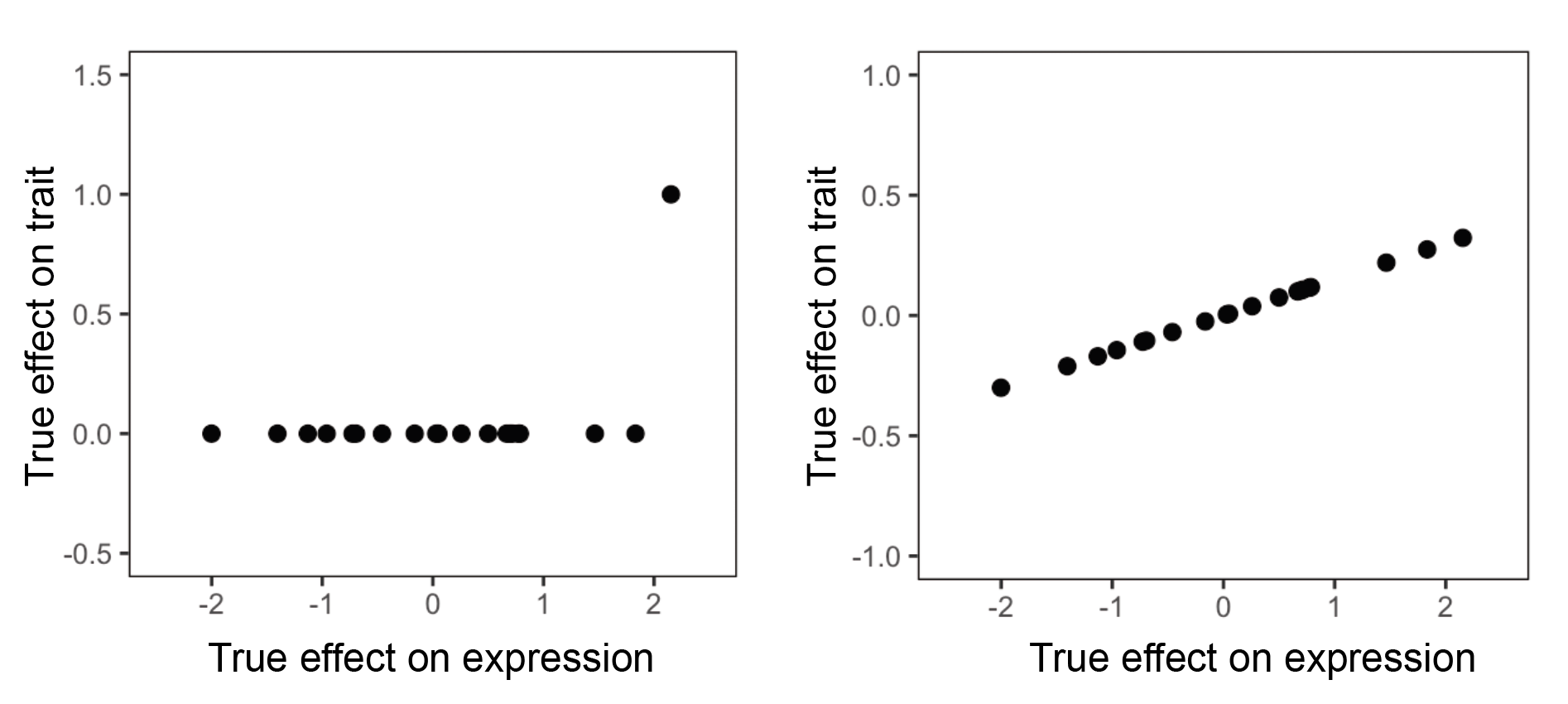
Here, we have two scenarios. Each point represents a SNP. In the left scenario, most SNPs affect the gene but have no effect on the trait other than a single outlier. In the right scenario, most most SNPs affect the gene and have proportional effects on trait. Which scenario do we think is more likely to implicate the gene’s expression as being relevant to the trait? Probably the one on the right, since if the gene truly exerts some causal effect on the trait, we would expect every SNP that affects the gene to also exert an effect on the trait. We think that the scenario on the left is much more likely to reflect pleiotropy, in which the single outlier SNP is affecting the trait through a mechanism that does not involve the gene.
It turns out that the scenario on the left, despite not reflecting what we perceive to be mediation of SNP effect on trait through the gene’s expression, will result in a substantial correlation between SNP effect on trait and SNP effect on the gene. This will cause this scenario to contribute to the overall estimate of \(\sigma^2\). However, the scenario on the left will not contribute to \(h_{med}^2\). Why? Because MESC involves regressing GWAS effect sizes on eQTL effect sizes, and the slope from we get from doing this will be very close to 0. To give some intuition for this, note that slope = correlation * SD(dependent variable) / SD(independent variable) (see the Wikipedia page on simple linear regression for discussion). In the scenario on the left, SD(dependent variable) is very small, which causes the slope to be close to 0. For the scenario on the right, we would expect this scenario to contribute substantially to both \(\sigma^2\) and \(h_{med}^2\).
To summarize, a key difference between \(\sigma^2\) and \(h_{med}^2\) is that the former basically looks at the correlation between GWAS and eQTL effect sizes, while the latter basically looks at the slope from regressing GWAS effect sizes on eQTL effect sizes. Although these quantities are often quite similar to each other, there are scenarios in which they won’t be (as outlined above). There is also the fact that when estimating \(h_{med}^2\), we go through a lot of trouble to split up SNPs by functional categories, so that we don’t get any spurious contributions to \(h_{med}^2\) arising due to systematically different non-mediated effect sizes in different functional SNP categories.
Is there anything wrong with \(\sigma^2\)? Of course not. I think that \(\sigma^2\) is a perfectly fine metric to quantify how “important” gene expression is to a disease, since importance is subjective and depends on what you want to learn from the data. However, I do believe that \(h_{med}^2\) comes much closer to the philosophical notion of mediation, in which we want to see how much SNP effect is specifically mediated through gene expression. I think that mediation is a good way to quantify the importance of gene expression, since mediation (as opposed to other causality scenarios such as pleiotropy) is how we conceptualize the involvement of gene expression in disease.
Reconciling MESC with our understanding of specific gene functions
This title is pretty vague, but hopefully it’ll make sense after you read this section. MESC involves regressing GWAS effect sizes on eQTL effect sizes across all genes. This is suggesting that if a SNP 1 has a certain effect on gene 1, and SNP 2 has a larger effect on a different gene 2, then on average SNP 2 will have a larger effect on the trait than SNP 1.
Hold on, why should this be the case? What if gene 2 has nothing to do with the trait? For example, let’s say that gene 1 is MYC (a really important gene), and gene 2 is RP11-195B21.3 (a random gene I found on google). MYC is much more likely to have a large effect on disease than RP11-195B21.3, so we would probably expect a SNP that affects MYC to have a much larger effect on disease than a SNP that affects RP11-195B21.3, even if the SNP’s effect on RP11-195B21.3 is larger.
Of course, the notion of eQTL effects being correlated with GWAS effects across genes doesn’t make any sense when you think of specific genes like this. However, in our case we are looking at averages across genes. We are basically saying that if we take all eQTLs of a given magnitude \(x\) (which will probably include many hundreds or thousands of genes), and we take all eQTLs of a given magnitude \(x + \epsilon \), then the average GWAS effect size of the second group will be greater than that of the first group. Indeed, for polygenic traits, in which many hundreds or thousands of genes are involved in the trait without many notable outliers, it makes sense to think about these averages. This is much more sensible than the two-gene scenario we described above.
(Thanks to Jesse Engreitz for helpful discussions regarding this point.)
Glossary
- eQTL: An eQTL is a SNP that is associated with the expression levels of some gene.
- Linkage disequilibrium: You can think of LD as correlations between nearby SNPs across individuals in a population.
- Heritability: If you’re not comfortable with thinking about heritability, please see my other blog post(s) on it. Briefly, you can think of heritability as the “total effect of genetics on a phenotype.” This quantity is often more straightforward to estimate than individual SNP effects on a phenotype, which are complicated by LD.
- Heritability enrichment: is related to the idea of “partitioning heritability,” in which we quantify how much total effect is coming from a particular set of SNPs (rather than the set of all SNPs). We are free to define this set of SNPs in any way that we want; for example, these SNPs can be located on a given chromosome, or be located in genomic regions annotated as carrying a particular histone mark, etc. The “heritability enrichment” of this set of SNPs is simply how much more heritability is coming from those SNPs than expected (a.k.a. if genetic effect was uniformly distributed across all SNPs). Enrichment for heritability means that more genetic effect on disease is coming from these SNPs than average, so we can interpret these SNPs as being more disease-relevant than average.
- Marginal vs causal: Sometimes I will refer to a GWAS or eQTL effect size as “marginal” or “causal.” A SNP’s “marginal” effect size is one that comes straight out of a GWAS. Due to correlations between SNPs, these effect sizes will “tag” the effects of nearby SNPs. A SNP’s “causal” effect size is its actual effect on the trait, which does not include these tagging effects. We typically cannot directly measure the causal effect size of a given SNP from GWAS, but there are some ways to get at SNPs with nonzero causal effects.
- Fine-mapping: is a way to try to identify causal GWAS hits or eQTLs in a region of marginal GWAS hits or eQTLs. Without going into detail, fine-mapping methods take into account the LD structure of a region of associated SNPs and give you a probability that a particular SNP truly has a causal effect on the trait.
- Colocalization: This concept is closely related to fine-mapping. One early way that people have tried to integrate eQTLs with GWAS was to simply intersect marginal GWAS hits with marginal eQTLs, but as you can imagine this is complicated by tagging effects of nearby SNPs. Colocalization involves jointly fine-mapping both the eQTL and GWAS hit in order to produce a probability that the exact same SNP is causal for both expression and trait.
- Transcriptome-wide association study (TWAS): TWAS was developed as an alternative approach to colocalization. Rather than looking for genes with one or more eQTLs that have a high probability of also being GWAS hits (as colocalization does), TWAS looks for genes with significant genetic correlation between their expression and trait. You can think of genetic correlation between two traits as the correlation between the SNP effect sizes for those traits. In other words, in TWAS, we want to see that when eQTL effect sizes for a given gene go up, then the GWAS effect sizes of those SNPs also go up.
- Mendelian randomization: Mendelian randomization (MR) is an approach that was developed a long time ago, but when applied to gene expression is very similar to TWAS. Whereas TWAS looks for correlation between eQTL effect sizes and GWAS effect sizes, MR looks at the slope when regressing GWAS effect sizes on eQTL effect sizes.
- TWAS vs MR: The conceptual difference between TWAS and MR basically boils down to the difference between correlation and slope (which as you can imagine are two very similar things). In practice however, there can be substantial differences between MR methods and TWAS methods, but these differences boil down to implementation details. For example, the most popular MR method for gene expression, SMR (Zhu et al. 2016), only looks at the top eQTL for each gene, while TWAS methods (e.g. PrediXcan (Gamazon et al. 2015) and FUSION (Gusev et al. 2016)) look at all eQTLs in the cis-locus (a.k.a plus-minus 1 megabase) around the gene. Conceptually, I think of these two types of approaches as doing basically the same thing.
- Colocalization vs TWAS/MR: TWAS/MR has various pros and cons relative to colocalization. For example, colocalization can eliminate scenarios where eQTLs and GWAS hits overlap due to “linkage,” whereas TWAS/MR cannot (in fact, colocalization was specifically designed for this task). On the other hand, TWAS/MR is more powerful than colocalization when a gene has multiple eQTLs that all overlap with GWAS hits.